The Coordinated Dollar
A Rigorous Analysis of Coordinated Capital — What One Dollar Can Do When It Is Never Interrupted, and Why the Coordinated Plan Outperforms a Lifetime of Good Decisions Made Separately
Certainty · Liquidity · Legacy
Living Asset Strategy series · The Coordinated Dollar · the Whitepaper — the complete reference layer, the deepest of four.
Every policy figure is drawn from one of three real carrier illustrations, every property figure from one professional analysis, every market figure from the S&P 500’s own published returns — reproducible, and never mixed across sources.
About This Analysis
This is the deepest layer of the Living Asset Strategy. The shorter pieces in this series are written to be understood on a first read; this one is written to be defended under interrogation. It is where the calculator lives — the place a skeptical CPA, a careful son-in-law, or a rival advisor can go to check that the intuition survives contact with the numbers. Most readers will never need it. It exists so that the claims in everything above it are earned rather than asserted.
It is worth saying plainly what this paper is not. It is not an argument that the market’s advertised return is the number to beat — because that number is not the number anyone keeps. The gap between a market average and what a real investor nets, after the four forces this series measures, is the whole subject of the companion Accumulation paper, The Actual Net Return, and Section 11 here takes it apart in full. This paper is not a defense of any branded system, and it is not an attempt to win a debate the reader never entered. What it argues is narrower, and I think more durable: that lifetime outcomes are decided less by the quality of any single piece than by how well the pieces are coordinated into one complete system. This paper does not tell you that you need any particular instrument. It shows what the coordinating jobs are, what it costs a household to leave them undone, and what changes when a single asset is positioned to do several of them at once — and it lets you draw your own conclusion about whether that is worth having.
The wealth builder and the business owner, whose capital is constantly being deployed and who feel the cost of having it in the wrong place. The professional with a large idle cash position who suspects it is costing more than it appears. The real-estate buyer who wants liquidity that cannot be frozen at the moment it is needed. The reader who has been told that whole life is a bad investment and wants to know whether the honest math actually says that. And the advisor who wants to see the calculation rather than take the conclusion on faith.
Every market figure in this analysis is a measurement, not a projection — drawn from the actual annual returns of the S&P 500 across its last full century, run through a single cash-flow engine. Every policy figure comes from one real carrier illustration for one real design, reproduced without adjustment. Where a number cannot be traced to either source, it is not printed. Where a claim cannot be measured, it is stated as directional rather than dressed up as precise. That discipline costs a few good sentences. It is what allows the rest of them to stand.
Executive Summary
The objective is the system, not the asset. A plan optimized to maximize the return on any single account runs unprotected into the first bad sequence at the wrong time. The real objective function is the quality and predictability of the complete-lifecycle outcome — what you accumulate, whether the income survives a poor sequence, and what completes and passes on. Rate of return is one input to that outcome, not the outcome itself.
A pile of good accounts loses to a coordinated system at identical returns. The loss hides in three seams: capital that earns nothing while it waits (a household with $1.25 million, $250,000 of it idle, earns a blended 6.4% rather than 8%); the absence of a second source to draw from in an ordinary down year; and the tax paid because no one decided which dollar should come from where. None of the three appears on a statement.
The honest benchmark is far lower than the advertised one. Across 2001–2025 — a generous quarter-century in which twenty of twenty-five years finished positive and the winners averaged 17.5% — the arithmetic mean was 10.32%. After the four compressions that act on every real dollar, the realistic investor kept a compound 4.93%: $332,750 on a $100,000 account, against the $1,164,870 the advertised rate implies.
One asset can hold several coordinating roles. A properly structured, dividend-paying whole life policy can serve as a reserve that earns while it waits, an account that does not fall when the market does, capital that keeps compounding while it is being used, and a legacy that completes itself the day it is in force. This paper follows one real policy — Marcus, age 42, $12,000 a year — through all four.
The Category 3 exhibit is the proof of dual use. A single representative rental property, purchased three ways, returns 7.28% for all cash, 14.84% on a conventional bank loan, and 29.09% when a $67,000 policy loan funds the down payment and $5,000 of the buyer’s own cash goes in — each figure a net annualized rate across the full fifteen-year hold, not a cumulative total. The property’s own cash flow repays that loan to the carrier, and the policy still reaches $581,400 of cash value and $1,013,303 of net death benefit by age 67. One dollar, two jobs, both traceable.
The conclusion is derived, not sold. The analysis goes where the honest numbers go: Section 9 runs Human Life Value precisely because that number often points toward term insurance rather than more whole life, and the paper follows it there. What the math points to, it names — and here it points to one instrument, because only one does all the coordinating jobs at once. A reader is left to draw that conclusion rather than told to; a system that only ever concluded “buy the thing I sell” would be a sales pitch with footnotes, and this is not that.
The Coordination Problem
1.0 The assumption underneath the assumption
Before any of the arithmetic, one premise has to be made explicit, because every plan rests on it and almost none states it: you live forward through uncertainty. The future is not a point. It is a range — and it is a range in two dimensions at once, both of which the ordinary plan quietly treats as fixed.
The first is how much the money will earn. No one is handed the sequence of returns in advance; the advertised average is a summary of a range, not a promise drawn from the middle of it. The second is when the money will be needed. A plan is built as though the timeline were known — twenty-five untouched years for the forty-two-year-old who retires at sixty-seven — but need does not keep to a schedule. A job ends, an opportunity appears, an illness arrives, a child needs help. The money is called on when it is called on, not when the plan expected.
You already believe this, and you can prove it to yourself by looking at any prudent portfolio: it holds bonds. Bonds are not there to out-earn the stocks — they do not, and everyone knows they do not. They are there to compress the range, to trade some of the average for reliability, so that the portfolio is usable in the particular year it is drawn on rather than merely acceptable on average. The moment you accept the bond, you have already conceded the whole of this paper's premise: that a resource has to be useful in the year you reach for it, not on average across years you may never see. (Statisticians have a name for the width of that range — standard deviation — but the name is not the point. The bond in your own portfolio is the point.)
Which sets the objective everything here is measured against. It is not the highest rate. It is to keep a family's resources useful across the whole range of futures that could arrive — available and productive whenever they are actually needed, with the least damage to the rest of the plan when they are drawn upon. Rate is an input to that objective. It was never the objective itself.
And it exposes the trade that the rest of this paper exists to examine. Every dollar you own lives somewhere, and every place it can live makes the same three-way trade: Growth, Safety, Access — you may have two, and you give up the third. Cash in the bank is safe and available but does not grow. The market grows but is neither safe nor reliably available in a bad year. A bond compresses the range but surrenders growth and is taxed as it goes. The question this whole body of work is built to answer is whether a single dollar can be made to hold all three at once — and if it can, what that dollar is worth to a plan that has stopped forcing the choice.
That is the coordination problem, stated at its root. The two families below are what it looks like in a life.
1.1 Two families
The greatest risk in your financial plan isn’t that you own the wrong things. It’s that the right things were never designed to work together.
Picture two families. They earn the same income. They invest in the same market, through the same three decades, and when the statements are totaled at the end, their average returns are nearly identical. They retire the same year.
Their retirements themselves look nothing alike — one anxious about every market swing and wondering how long the money will actually last, the other largely untroubled by either, because the income does not depend on what the market did that year. And at the end, they leave their children two completely different futures.
One family retires and never carries the anxiety the other lives with. When the market falls hard early in their retirement — and for one of them, it does — their income doesn’t flinch. When the second passes, the children don’t inherit what the other family’s children will: an account drawn down by a bad decade, a tax bill on what is left, and no one whose job was to see the whole. They inherit a head start instead — capital already working, decades of compounding already done, a place near the top of a climb the other family’s children are just beginning at the bottom.
The other family did nothing wrong. They saved. They invested. They earned the same returns. But their money worked as a pile — a collection of separate accounts that never spoke to each other. So an ordinary down year forced them to sell at exactly the wrong moment. Their taxes ran higher than they needed to, year after year, because no one ever coordinated which dollar came from where. And what was left at the end was smaller, later, and less certain than it might have been.
The difference wasn’t the investments. Both families earned the same market return — this is not a story about one portfolio beating another. It is a story about what happened to two identical returns after coordination acted on one of them and not the other. One family’s money worked as a single system. The other’s worked as a pile.
That is easy to claim and hard to believe — at the same returns? — so the rest of this paper puts the two families’ accounts side by side and shows, in dollars, where the coordinated one pulls ahead. Not with better performance. With better architecture.
At the same returns.
1.2 What “coordinated” actually means
The word is doing precise work, so it is worth defining before it is used another hundred times. A coordinated plan is one in which the right amount to hold in any position — a policy, an annuity, an equity sleeve, a cash reserve — is determined by the net, all-phases outcome of the complete plan, and never by comparing that position’s standalone return to another’s.
That definition has an immediate consequence. It means the familiar objection — the policy earns about five percent and the market earns about ten, so why would anyone choose the policy — is not a wrong answer. It is a wrong question. It is an asset-level comparison offered as though the assets lived alone. They do not. They live in a household, across three phases, over fifty years, and what each one is worth depends on what it lets the others do.
The word also carries an honest diagnosis. “Coordinated” means the parts of a plan are made to work as one system rather than sitting side by side — the accumulation, the income, the tax exposure, the legacy, and the instruments that serve them. For most households I work with, some of those pieces already exist and are simply uncoordinated; almost as often, a piece the plan genuinely needs is missing entirely and has to be added. Coordination is not a promise that you already own everything required. It is the discipline of building the whole so the parts reinforce rather than undercut each other — which sometimes means organizing what you have, and sometimes means adding what the plan is missing.
1.3 Return is an input; the coordinated outcome is the objective
Rate of return — call it ROR, ROI, or IRR — is a solution, not the solution. It is one variable inside the real objective function, which is the quality and predictability of the complete outcome: accumulation, plus a sequence-protected distribution, plus a legacy that completes on time. A plan tuned only for accumulation return accepts a hidden fragility, and a single large loss at the wrong moment erases years of the edge it was optimizing for.
A coordinated plan is optimized for the whole life of the money — the result the household actually lives on and leaves behind — not for a single headline accumulation number. The right allocation to any instrument is the output of that optimization, sized to the household — not an input to be defended against a benchmark.
This has a second implication that most of the whole-life and Banking Concept marketing world — call it this category throughout — consistently misses. If the value of an asset is its role in the system, then a value proposition built on that asset out-returning something else is rented from the market’s mood. A good year takes it back. I have watched it happen: a client persuaded by a returns argument, who cancelled a few years later when the market cooperated and the argument he had been given no longer seemed to hold. Nothing about the policy had changed. Only the story he had been told about why he owned it. So this paper is built on claims a good year cannot refute — certainty, role, and time horizon — and not on the claim that the instrument beats anything.
1.4 What this analysis is, and is not
- It is not an argument that the policy wins a rate contest against the market’s advertised return. That contest is the wrong one — the advertised return is not what a real investor nets, as this series measures in detail — and Section 11 shows exactly where the honest, kept numbers land, without rounding in the policy’s favor.
- It is not an argument against market investing, or against paying for advice. Both are load-bearing parts of a coordinated plan.
- It is not a defense of any branded system. Where this category has overclaimed, Section 12 says so plainly and corrects it — including the claims that are most often made in the instrument’s favor.
- It is an argument that coordination is the principle, that the principle is universal, and that this particular instrument happens to be an unusually efficient way to implement it — for the households where it fits.
The Hidden Cost of a Pile
A pile of good accounts quietly loses to a coordinated system — even when every account in the pile performs identically to its counterpart in the system. The loss does not show up on any single statement. It hides in the seams between them. There are three seams, and each one costs real money.
2.1 Seam One — capital that earns nothing while it waits
Take a household with $1.25 million. A million of it sits in growth assets earning 8%. The other quarter-million sits in cash — an emergency fund, a reserve, dry powder for the next opportunity: the household's Opportunity Fund — earning next to nothing.
That household will tell you it earns 8%. It does not.
| Position | Balance | Rate | Weighted contribution |
|---|---|---|---|
| Growth assets | $1,000,000 | 8.00% | 6.40% |
| Cash reserve | $250,000 | ~0.00% | 0.00% |
| Blended portfolio | $1,250,000 | — | 6.40% |
The idle reserve is not free. It costs the household roughly a point and a half of blended return, quietly, year after year — and nobody feels it, because the cash was “supposed” to earn nothing. That is the price of holding a necessary thing in an isolated place.
Now move that same reserve — without giving up a dollar of access to it — into a position that earns a contractual mid-single-digit rate and can still be drawn against on demand.
| Position | Balance | Rate | Weighted contribution |
|---|---|---|---|
| Growth assets | $1,000,000 | 8.00% | 6.40% |
| Reserve, repositioned | $250,000 | ~5.00% | 1.00% |
| Blended portfolio | $1,250,000 | — | 7.40% |
Nothing was risked. No new market exposure was taken. Nearly a full point of blended return was recovered from money the household had already set aside and written off — and that point compounds for decades.
That $250,000 is an abstraction. Here is the version that is not. You almost certainly keep an emergency fund — three to six months of expenses, sitting in a savings account, earning next to nothing. Every sound financial plan tells you to hold it, and that advice is correct. What no one tells you is that holding it in a bank account is a choice, and that the choice has a price.
The reserve has to be safe and it has to be reachable. It does not have to be idle. A properly structured policy can hold the same reserve — safe, and reachable on demand through a policy loan or withdrawal — while it earns a contractual return instead of nothing. Same dollars, same safety, same access. One version earns zero. The other works the entire time it waits.
In practice this is a matter of preference, not prescription. Some of the households I work with like to keep a single month of expenses in the bank and the rest of the reserve in the policy; others prefer two or three months in cash and the remainder in the policy. Once retired, most move to holding roughly a year of expenses in reserve, structured the same way. The right split is the one that lets a person sleep — and in every version of it, the majority of a reserve that was going to sit there anyway is finally earning something.
This is the cleanest on-ramp to an idea the rest of this paper develops in full — that the question is never merely whether capital is safe, but whether safe capital is being put to its highest use — the most productive job it could be doing without giving up the safety or the access. Almost no one has ever looked at their emergency fund and called it a cost. It is one. It is also the easiest cost in a plan to recover, because nothing about the money’s safety or availability has to change — only where it sits.
Moving the reserve is the smallest thing this asset does — and it already pays for itself.
Be clear about what has and has not just been claimed. Recovering that point is the first and least ambitious use of the instrument: capital the household had written off as dead now earns contractually while remaining available on demand. It requires no deal, no opportunity, and no judgment about anything. It is the floor of the argument, not the ceiling.
What the capital does once it is positioned there is the subject of most of this paper. The same dollar is borrowed against to buy a building and to expand a business while it continues compounding. It stands behind a death benefit from the first premium. It becomes the account a retiree draws income from in the year after the market falls, so the portfolio is left alone to recover. And Section 7 describes a man whose income rose sharply within two years of implementing — not only because of the policy’s return, but because the certainty freed his attention to do his work. None of that is inside the point recovered here. All of it is on top of it.
One honest note on the arithmetic above: it is a weighted-average illustration, not an engine output. The rates are round numbers chosen to make the mechanism visible. The mechanism itself is not an approximation — a portfolio’s blended return is the weighted average of its parts, and a zero-yielding slice drags the whole in exact proportion to its size.
2.2 Seam Two — no second source in an ordinary bad year
Markets have down years. That part is ordinary, expected, and not the story. The story is what a structure does when one arrives.
A retiree drawing income faces a risk that has nothing to do with their average return: the order the returns arrive in. During accumulation, order is irrelevant — reorder twenty-five annual returns any way you like and the ending balance does not move a dollar, because multiplication is commutative. The moment withdrawals begin, that stops being true, and order becomes the dominant variable.
Consider the household this paper returns to throughout: $1,000,000 in a Tax-Deferred account, withdrawing $48,000 a year — which, at the 25% combined effective rate used everywhere here, puts $36,000 of spendable income in their pocket. Now suppose an ordinary down year — not a crash, the kind of year the market delivers roughly one in four. The portfolio falls 15%, and the retiree still needs the year’s income.
| Step | Value |
|---|---|
| Starting portfolio | $1,000,000 |
| After an ordinary 15% decline | $850,000 |
| Less that year’s $48,000 income | $802,000 |
| Gain required simply to return to $1,000,000 | 24.7% |
Read that last line slowly, because it is the entire point. A routine 15% year — not a catastrophe, not a once-in-a-generation crash — already demands a 24.7% rebound just to get back to even, and it gets worse if the next year’s income is drawn before the recovery arrives, which of course it is. Nothing improbable happened here. This is a normal year doing permanent damage, because the shares sold at a discount to fund living expenses never participate in the recovery. The portfolio is structurally smaller for every future year. The same set of returns that produced a fine accumulation outcome produces attrition in distribution — and it does not take a disaster to start it.
Here is the part that matters, and the part most explanations get wrong. In the down year itself, both families take that year's income the same way — from the portfolio — because no one knows in advance how a year will end; you cannot decide in January to spare a portfolio you don't yet know will fall. The difference appears the following year, once the loss is a fact. The family with only a pile has no second option: next year's income comes out of the portfolio again — selling more shares, now at the discounted level, locking in the damage and making the 24.7% recovery a nearly impossible task. The family with a coordinated system does something different: in the year after the loss, it draws income from a position whose value did not fall with the market — the policy's cash value — and leaves the portfolio untouched so the recovery works on the whole balance, not a depleted one. It returns to drawing from the portfolio once it has recovered. Same market, same returns, same ordinary bad year. One structure has an answer for the year that follows it; the other does not. The full anatomy of that risk — how the order of returns governs a retirement, and how large a buffer the historical record actually demands — is the subject of the companion Distribution paper; this paper takes it only as far as the seam requires.
And you cannot build that second position after the bad year arrives. The option either exists at the start of the year following a loss or it does not — and whether it exists was decided years earlier, while you were still working. That is the whole reason an accumulation-phase decision cannot be graded on accumulation-phase return. It is like grading a bridge support on how much it weighs rather than on whether the bridge stands.
2.3 Seam Three — the tax paid because nothing was located deliberately
Every dollar you own lives at a tax address: Taxable (also called non-qualified), Tax-Deferred, or Tax-Free. A pile ignores the addresses; it simply holds assets. A coordinated system decides, deliberately, which dollar grows where, which dollar funds income first, and when the tax is paid — and when it is not. The pile pays whatever falls out of the structure. The system generally pays closer to the least the law allows. Across a retirement, that gap is not rounding. It is years of income.
2.4 The seams compound — and nobody is accountable for the total
Three seams. None of them appears on a statement. Every one of them is a cost of structure, not of performance. And the reason they persist is not a conspiracy. It is that no one is accountable for the whole. The custodian minds the account. The fund company minds the fund. The CPA minds April. Every layer is administered by someone doing their own job competently, and nobody is standing over the total, asking what all of it compounds to across a lifetime.
That absence — not any single decision — is the real cost. An uncoordinated plan leaks at every seam, and the leaks compound. So the honest question is no longer “which investment is best?” It is: what would it look like if the pieces actually worked as one system — and what would hold a system like that together?
The Honest Benchmark
Before any instrument can be evaluated, the thing it is being measured against has to be stated honestly. This section derives that number from scratch. It borrows nothing on faith.
3.1 The advertised number and the kept number
Take the twenty-five years from 2001 through 2025 — the primary accumulation window for a great many people reading this. Twenty of those twenty-five years finished positive. The positive years averaged 17.5% apiece. Only five finished down. This was not a punishing quarter-century; it was a generous one.
The arithmetic mean of those twenty-five annual returns is 10.32%. That is the number a projection uses. Applied to $100,000 over twenty-five years, it implies an ending balance of $1,164,870.
A real investor in that same market, in a Tax-Deferred account, holding an ordinary advised portfolio, ended the period with $332,750.
Same market. Same twenty-five years. A gap of $832,120 — produced not by any single crash but by ordinary years. Every twenty-five-year stretch in the record contains positive years and negative ones together, and it is their combined arithmetic — not a bear market alone — that opens the gap.
3.2 Where the difference goes — four compressions, measured
The gap is not caused by the bad years. It is caused by four forces acting on every year, the good ones included. Each one is measured, not assumed.
First, volatility. The arithmetic mean of a volatile series always exceeds the rate at which money actually compounds. This is not opinion; it is arithmetic. The size of the gap depends on the actual ups and downs of a given stretch — the more violent the swings, the wider it opens. Across the S&P 500’s last full century (1926–2025) the arithmetic mean was 12.11% and the compound rate was 10.28% — a measured gap of 1.83 points a year. Over the specific 2001–2025 window used here the gap was 1.58 points: the arithmetic 10.32% compounds at 8.74%. (The two figures differ because the drag is not a fixed constant; it is whatever the actual sequence of returns produced.)
Second, activity. An index return is what a dollar receives when it is left alone, and almost no dollar is left alone. Between the index and the investor stand two layers of activity — a fund manager acting on the money, and the investor acting on it in turn — and each, on average, subtracts from what the index would have delivered. This is Activity Drag: the cost of an active dollar. It arrives in two separately measured parts.
The larger part is structural, and it requires the investor to do nothing wrong at all. Most retirement money does not sit in a bare index fund; it sits in actively managed funds, the default in most 401(k)s. Over the twenty years through 2024, roughly 92% of active large-cap funds trailed the S&P 500 (S&P Dow Jones Indices’ SPIVA scorecard). Nor is that a fringe way to invest: as of the end of 2025, roughly 46% of U.S. fund assets — about $16 trillion — were still held in actively managed funds rather than index funds. Nearly half of every fund dollar in the country is placed with a manager who, in large-cap equity, trails the index in nine years out of ten, before its owner makes a single decision. The manager was active on the saver’s behalf, and the activity cost them.
The smaller part is the behavior gap: the return an investor captures falls short of the return their own funds earned, because real people move money at imperfect moments — pausing contributions when a downturn makes the future feel uncertain, resuming once it has passed. Morningstar’s Mind the Gap measures the aggregate effect at about 1.2 points a year over the decade through 2024. This is the part properly called timing, and it is both the smaller leg and the more contested one: recent peer-reviewed work in the Financial Analysts Journal argues the gap is substantially a mechanical artifact of how cash flows are measured rather than evidence of mistiming. I name that dispute rather than lean on it, because the case does not need it.
This analysis applies 1.5 points, and it rests on the structural leg rather than the behavioral one — a modest assumption against a record in which nine of ten active funds trail their benchmark. That anchoring matters for a second reason: a critic can fairly argue the behavior gap exists only because markets move, and that stacking it on Force One charges one risk twice. Manager underperformance is not caused by volatility and would persist in a perfectly calm market. Anchored there, this force does not depend on the component that objection targets. It moves 8.74% to 7.21%.
Third, tax. A 25% combined effective rate — roughly 20% federal and 5% state — applied at the end of the period costs about 1.22 points of annualized return, taking 7.21% to 5.99%.
Fourth, fee. Every investor knows the fee they were quoted. Almost none can state the fee they actually pay. A broad index fund’s own expense ratio runs three to seven basis points — real, and genuinely small. Beneath it sits the advisory fee, usually around 1%, and beneath that sit the layers almost nobody is shown: trading costs inside the funds, revenue sharing and platform fees, the drag of uninvested cash. Once every layer is counted, the all-in cost for a typical advised investor lands at or above 1.0% a year; comprehensive managed arrangements run to 1.5% and higher. This analysis uses 1.0% — the conservative end of that range. A 1.0% fee charged on the balance every year costs slightly more than 1.0 point of annualized return — here, 1.06 points, taking 5.99% to 4.93% — because the fee is levied on a growing balance and each dollar it removes can no longer compound in any later year. A flat 1% deducted annually always compounds into a somewhat larger drag on the final annualized figure; that is why the number is 1.06 and not exactly 1.00.
| The compression, in order | Annual rate | Ending balance on $100,000 |
|---|---|---|
| Average Gross Return (arithmetic mean, 2001–2025) | 10.32% | $1,164,870 |
| less volatility (measured) | 8.74% | $812,153 |
| less activity (1.5%, conservative) | 7.21% | — |
| less tax (25% terminal) | 5.99% | — |
| less all-in fee (1.0%) | 4.93% | $332,750 |
| Actual Net Return | 4.93% | $332,750 |
Two observations that survive scrutiny. The fee is the smallest of the four forces — about 1.06 points — and it is the only one you actually choose. You cannot vote a bear market out of existence, you cannot fully cure the ordinary human response to a red screen, and you cannot repeal the tax code. You can decide what you pay to invest. And the timing force is not a story about a careless investor: its larger component has nothing to do with the investor at all.
3.3 Every window in history
A fair objection: one twenty-five-year window is one draw. So all four forces — with the fee held at the same 1.0% — were run across every rolling twenty-five-year window in the century — seventy-six of them, from the window beginning in 1926 to the one ending in 2025.
| Across 76 rolling 25-year windows | Actual Net Return | Ending on $100,000 |
|---|---|---|
| Worst window (1929–1953) | 1.46% | $143,751 |
| 10th percentile | 4.00% | — |
| 25th percentile | 5.45% | — |
| Median | 6.40% | $472,014 |
| 75th percentile | 8.77% | — |
| 90th percentile | 9.77% | — |
| Best window (1975–1999) | 13.13% | $2,185,661 |
Two findings matter. The first is that the compression is not an artifact of the window chosen: it was positive in seventy-six of seventy-six windows, never narrower than 4.7 points and, in the frothiest windows, as wide as 7.0. The two published medians make the typical case reproducible by subtraction — a median Average Gross of 11.8% became a median Actual Net of 6.4%, a shortfall of roughly 5.4 points for the typical window. There is no quarter-century in the record where the advertised number and the kept number were close.
The second is how widely outcomes are spread. A median of 6.40% sits between a worst case of 1.46% and a best of 13.13%. Planning to the midpoint while ignoring how far real outcomes spread on either side of it is not optimism. It is a risk-management failure. And no one chooses their starting year.
3.4 What this does and does not prove
It does not prove that markets have no place in a plan. It proves something narrower and more useful: the number in the brochure is not the number you keep, the difference is large and measurable, and any plan built on the brochure figure is built on a number that has never once shown up in a real investor’s account. That is the benchmark against which every other instrument in this paper is measured.
The Instrument the Seams Point To
4.1 The specification, before the name
Set the products aside and write down what Section 2 requires. A coordinated plan needs a position that:
- earns while it waits — a meaningful contractual rate, so reserve capital is never idle;
- does not fall when the market falls — so that in the year after a loss, income can be drawn from it while the portfolio recovers;
- is reachable on demand and grows tax-free — accessible without application, approval, or the possibility of being called, and reached in a way that is not a taxable event and does not raise the tax on Social Security or trigger IRMAA;
- keeps compounding while the capital is being used elsewhere — the same dollar working in two places at once;
- settles the plan’s protection and legacy obligations on the day they come due, whenever that is, income-tax-free to those who receive it.
Nothing in that list mentions insurance. It is a specification, and it is what the three seams demand. Only one widely available instrument satisfies all five at once — and the tax treatment woven through the list is not a footnote to it but a central part of what each of those jobs is worth.
4.2 Naming it honestly
The Living Asset Strategy is built on properly structured, dividend-paying whole life insurance from a participating mutual carrier — the same financial instrument behind what some call The Banking Concept. I name that plainly, and early, because a paper that concealed its own mechanism would forfeit the standard it is written to meet. What separates this analysis from the marketing that surrounds the category is not the instrument. It is that we use the mechanics, not the playbook — and in Section 12 we correct the category’s own overclaims before any critic has to.
If you tensed at the words “whole life,” that reaction is earned. Most of what is said about this instrument, in both directions, is argued at the wrong altitude — comparing one asset’s return to another’s. What follows measures something different: what one asset does to the behavior of an entire system across fifty years.
4.3 What “properly structured” means
Not all whole life policies are the same instrument, and the difference is not marketing. There is a design dial. At one end sits a protection-maximized policy: all base premium, the largest possible initial death benefit per dollar, and very little early cash value. At the other end sits a cash-maximized policy: a modest base, a substantial paid-up additions rider, and as much early accessible cash value as the tax code permits.
The legal edge of that design space is the Modified Endowment Contract line. Cross it and loans and withdrawals lose their favorable tax treatment. “Properly structured” means engineered deliberately close to that line, and under it.
There is an irony in this design that the category’s own marketing routinely drops, and it matters. Minimizing the initial death benefit is not a rejection of the death benefit — it is the most efficient long-run path to it. Every paid-up addition purchases a small, fully paid-up slice of coverage, and dividends buying further additions compound the effect. The cash-maximized design generally produces more death benefit by the age death is actually likely to occur. Living benefits and death benefit are the same contract seen from two ends of time. Cash value is, actuarially, the present value of the future death benefit. You cannot have uninterrupted compounding, contractual loan collateral, and tax-advantaged access without the insurance chassis that the death benefit represents.
Candor about incentives, since it is the fastest way to earn a skeptical reader’s trust: agent compensation is driven almost entirely by base premium. A cash-maximized design pushes most of the premium into the additions rider, which pays a fraction of that. The gap is not small. In a recent case, the properly structured design paid the agent about 18.8% of what an all-base policy would have on the identical premium — roughly eighty percent less. The design that serves the client best pays the advisor least. That misalignment is precisely why badly structured policies exist, and it is why a buyer who screens on structure before anything else is behaving rationally. Structure is where this is won or lost.
And structure is only the beginning. A policy built for the Banking Concept is not a set-it-and-forget-it purchase; it is an instrument that has to be managed for as long as it is used. The MEC line is not a wall you clear once at issue — it is a moving boundary that every loan, repayment, dividend, and paid-up-addition can push against, and a single misstep converts the contract to a Modified Endowment and forfeits the tax treatment the entire strategy depends on. The premium-offset election has to be timed, the dividend option chosen deliberately, the funding kept in its proper range as the policy is used. None of this is difficult in the hands of someone who does it routinely — but it is not automatic, and it is not something a policy does by itself on a shelf. It is the ordinary, ongoing work of keeping a well-built instrument well-run, and it rewards an advisor who has managed many of these over years rather than sold a few. This is the second reason the instrument is not separable from the advisor who stands behind it. The first is getting the design right. The second is keeping it well-run over time.
4.4 Marcus
Every figure that follows comes from one real illustration for one real design. Nothing is scaled, averaged, or invented.
| Parameter | Value |
|---|---|
| Insured | Marcus — male, age 42, Preferred Plus Non-Tobacco |
| Annual premium | $12,000 |
| Initial total death benefit | $251,264 |
| Dividend option | Paid-Up Additions |
| Tax status | Non-MEC, by design |
| Carrier | A participating mutual insurer founded in 1847 |
The structure is the point. Roughly two dollars of rider face for every dollar of base face is what allows the paid-up-additions dollars to go in without tripping the MEC line — the maximum early cash value the tax code allows, in a contract that still carries a quarter of a million dollars of protection from day one.
4.5 The capitalization period, honestly
The most common objection to this instrument is that it takes years to build — that the early years are dead money. For a poorly designed policy, that is largely true, and it is worth saying so before a critic does. There is no honest design in which all of your money is working from day one; first-year accessible cash value runs roughly 70 to 80 percent of premium. This is infrastructure, and infrastructure is capitalized before it produces.
So let us look at what this particular design actually does, against the simplest possible alternative: putting the same $12,000 a year into a bank account.
| Year | Cumulative premium paid | Same money saved in a bank | Policy cash value |
|---|---|---|---|
| 1 | $12,000 | $12,000 | $9,714 |
| 2 | $24,000 | $24,000 | $20,401 |
| 3 | $36,000 | $36,000 | $32,553 |
| 4 | $48,000 | $48,000 | $45,783 |
| 5 | $60,000 | $60,000 | $60,021 |
| 6 | $72,000 | $72,000 | $74,977 |
| 7 | $84,000 | $84,000 | $90,774 |
| 10 | $120,000 | $120,000 | $143,657 |
| 15 | $180,000 | $180,000 | $255,851 |
| 20 | $240,000 | $240,000 | $402,130 |
| 25 | $300,000 | $300,000 | $593,235 |
By year five the cash value ($60,021) has caught the cumulative premium ($60,000). The break-even arrives at year five — not the “five to ten years” the generic objection assumes, and not the decade the harshest version claims.
Now put a number on it. Suppose Marcus needs $67,000 for something — a down payment, an opportunity. Saving it at $12,000 a year in a bank account takes 5.58 years. This policy’s cash value crosses $67,000 at roughly 5.47 years — essentially the same timeline, marginally sooner, and only because the policy is compounding while the bank account is not.
The timeline is not the difference. It takes about the same time to build the money either way. The difference is that the policy dollar carried $237,000 of protection the entire time it was building — and, once borrowed against, the underlying cash value continues to grow during the life of the loan.
The “dead money” objection assumes Marcus is choosing between the policy and saving. He is not. He reaches the same milestone on the same timeline, and several other jobs get done along the way.
The Four C’s
The mechanics have a shape, and it echoes the words on the door: Certainty · Control · Compounding · Continuity. The first three teach the living mechanics. The fourth is where they add up across time, and the paper arrives at it deliberately.
5.1 Certainty
Certainty answers Seam Two, and it is the soul of the instrument. Marcus’s cash value has a contractual floor and grows on a guaranteed-plus-dividends basis. It does not move with the market — not up with it, and not down with it. That non-correlation is precisely what makes it usable as the position a household draws income from in the year after a loss, while the portfolio recovers. An asset that fell alongside the portfolio would be no help at all.
Non-correlation is usually described against the market — the cash value does not fall when stocks do. But there is a second axis, and for a retiree it may matter more: this asset is also non-correlated to tax-rate risk.
Income drawn properly from a policy does not enter the figure the tax code calls modified adjusted gross income. That one fact has consequences that ripple through a retirement. Because the income does not land in that figure, it does not push Social Security benefits further into taxation, and it does not lift a household across the thresholds that trigger the Medicare surcharges known as IRMAA. Other income sources do both, whether or not the tax on them is high.
This is where a distinction most people have never been shown becomes sharp. A number of assets are called “Tax-Free” and are not free of this second effect. Municipal bond interest is the familiar example: it escapes income tax, yet it still counts toward the modified-adjusted-gross figure, so it can still raise the tax on Social Security and still push a household into a higher Medicare bracket. Properly structured policy income does neither. It is not merely taxed favorably; it sits outside the machinery that turns other income into higher taxes and higher premiums elsewhere.
The full weight of this lands in the distribution years, where the interaction of income sources, brackets, surcharges, and Social Security taxation is its own subject — and the companion Distribution paper is where it is taken up properly. What belongs here is only the principle: an asset can be non-correlated to the market and non-correlated to the tax environment at once, and the second kind of independence is rarer, and rarely discussed.
It is worth being exact about what is contractual and what is not, because the loose word “guaranteed” is where this category loses careful readers. The dividend scale on a participating policy — currently about 6.00% — has two components:
- The guaranteed interest rate. Typically 2–4% depending on carrier and contract. Contractually locked for the life of the policy. It cannot change, up or down, once the contract is in force, and it applies to every dollar of cash value regardless of the insurer’s investment performance.
- The excess dividend. Currently around 3% on this carrier. This is the non-guaranteed component, and it moves with the insurer’s investment results, mortality experience, and operating efficiency.
It is worth being precise about exactly what “non-guaranteed” touches, because the word frightens people out of the category for the wrong reason. It does not mean the cash value can fall. Once a dividend is credited and once interest is credited, that value is locked in and cannot be taken back — the contract has a floor that only rises. The non-guaranteed element applies solely to each future year’s excess dividend: whether it is paid, and how much. A lower dividend in some future year means the cash value grows a little more slowly that year — never that it declines. There is no market mechanism inside this contract that can subtract from a balance already credited. So the only thing at risk is the rate of future growth on the excess portion, not a single dollar of the cash value already built.
So roughly half of the policy’s long-run return rests on a rate that cannot be reduced. The relevant question for the other half is how reliable it has been. The carrier in this illustration was founded in 1847 and has paid both the guaranteed interest and an excess dividend on top of it in every year since — an unbroken record through the Civil War, the Great Depression, two world wars, the stagflation of the 1970s, 2008, and the pandemic. Not one missed year in the whole of it. A second major mutual insurer, founded in 1851, holds the same unbroken record. Two carriers, two centuries, no missed year between them.
The honest framing is therefore neither “guaranteed” nor “speculative.” It is that the contractual portion cannot be reduced, and the non-guaranteed portion has been paid in every year of a century and three-quarters, across every major economic disruption in American history. That is a claim about direction, not about rate — and stating it that way is what lets it survive the follow-up question.
For context, the same carrier’s published dividend interest rate since 1989:
| Period | Dividend interest rate range |
|---|---|
| 1989–1994 | 9.20% – 9.93% |
| 1995–2003 | 6.48% – 8.50% |
| 2004–2018 | 5.74% – 6.34% |
| 2019–2026 (current) | 5.75% – 6.34% |
The illustration in this paper uses a scale near the bottom of that range. That matters for Section 11, and it cuts in the reader’s favor.
There is a mechanism under that unbroken record, and stating it plainly is what turns the bond-replacement claim from an assertion into a demonstration. A participating policy's growth is the dividend, and the dividend is the policyholder's share of the mutual company's profit. In a mutual company there are no outside shareholders; the policyholders are the owners, and the profit is theirs.
That profit comes from two sources, and they stack. The first is the carrier's own investment return — and here is the fact that matters most for this section: a mutual insurer's general account is invested overwhelmingly in high-grade bonds, roughly three-quarters of it. When you hold cash value, you are already holding, indirectly, a professionally managed, century-scaled bond portfolio — one larger and better-priced than any a household could assemble. The second source is underwriting profit: every line the company writes — term, disability, annuities, long-term care — is priced to bring in more than it pays out, or the company stops writing it. Both streams flow into the same pool, and the owners share it.
Two consequences follow, and both matter. First, this is why the dividend is not — as the loudest critic of this category insists — merely a refund of an overcharged premium. A refund cannot exceed what you paid, and it cannot depend on the performance of business lines you never bought. The dividend does both: it can and does exceed the policy's own cost, and it rises and falls with the profit of the whole company. It is an ownership distribution, not a rebate. Second, because it is an ownership share, its size tracks ownership — the more cash value a policy holds relative to its death benefit, the larger the owner's stake, and the larger the share. That is precisely why a properly structured, cash-maximized design is built the way it is.
So when this paper compares cash value to a bond, it is not a strained analogy. The cash value is funded by a bond portfolio — plus an underwriting profit the bond investor never receives — wrapped in a contractual floor, tax deferral, and uninterrupted access the bond does not have. The comparison that follows is bond-to-bond at its root, and the policy's version carries advantages the raw bond cannot.
There is a formal result behind the intuition, and it is not from the insurance industry. Kenneth Arrow — a Nobel laureate in economics — posed a puzzle: in expected-value terms every insurance contract is zero-sum, so why does insurance rationally exist at all? A resolution published in 2023 in the Annals of Actuarial Science, a peer-reviewed actuarial journal, shows that when parties are evaluated by the growth rate of their own wealth through time — rather than by an average across hypothetical parallel worlds — an insurance contract can raise the time-average growth rate of buyer and seller simultaneously. A contract that expectation-thinking calls a pure cost can be, mathematically, win-win.
The underlying mathematics is uncontroversial and is the same arithmetic that produced the volatility measurement in Section 3: a volatile path compounds more slowly than its own average suggests, so reducing the variance of a path can raise what it actually compounds to, even after paying for the reduction. That is the economic case for certainty, stated without slogans. It is also why a value proposition built on certainty cannot be refuted by a good year in the market — it never rested on the market to begin with.
Here is the comparison that matters, and notice which comparison it is not. The cash value is not being measured against the market. It is being measured against the bond — the position a prudent household already holds, and holds for exactly the reason Section 1.0 described: to compress the range, to be the reliable, drawable money that does not fall when stocks do. The policy's cash value does that same job. The question is only which instrument does it better, dollar for dollar, once tax is counted honestly.
Take a $100,000 safe sleeve — $72,000 in bonds, $28,000 in cash — the stabilizing money a prudent household already holds, and carry it for a twenty-five-year retirement. For the bond, use what high-grade corporates yield today — about 5.4% (Moody's Seasoned Aaa Corporate Bond Yield, as published by the Federal Reserve Bank of St. Louis), held in a bond fund at the average bond-fund fee of 0.36% (Investment Company Institute, 2025); for the cash, about 3.0% over the long run, at no fund fee — both taxed annually at the 25% effective rate this paper uses throughout. For the policy, use the same illustrated 5.00% that Section 11 holds it to. Spell the sleeve out, nothing hidden inside a blended average:
| The safe sleeve, spelled out | Bonds · $72,000 | Cash · $28,000 |
|---|---|---|
| Gross rate | 5.4% | 3.0% |
| Less fund fee | −0.36% | — |
| Less income tax, every year | −25% of the gain | −25% of the gain |
| Net rate it actually keeps | 3.78% | 2.25% |
| After 25 years | $182,043 | $48,836 |
The bonds keep 3.78%, the cash 2.25%; blended, the sleeve grows to $230,879 — a net 3.40% a year. Hold that same $100,000 in the policy's cash value instead — same safety, still reachable on demand, no fund fee and no annual tax:
| $100,000 safe sleeve · 25 years | Net rate | After 25 years |
|---|---|---|
| Bonds + cash, as typically held | 3.40% | $230,879 |
| Policy cash value | 5.00%, Tax-Free | $338,635 |
Read the rates before the results, because that is the whole point. The bond yields more on paper than the cash value — a 5.4% headline against 5.00% — and still finishes far behind. Its 5.4% is before the fund fee and the tax it owes every year, so what it actually keeps is 3.78%, while the policy's 5.00% is already net and Tax-Free. Same safety, same access, $107,756 more. And the gap does not close by moving the whole sleeve into bonds and holding no idle cash at all: even then the most it keeps is $252,838 — still $85,798 short of the policy's $338,635 — because the bond is charged a fee and taxed every year it works, and the cash value is not.
And the cash value does two things the bond cannot. It carries a contractual floor beneath the illustrated figure, so its range is compressed from below in a way the bond's price is not when rates move against it. And it remains fully available the entire time — borrowable against on demand, uninterrupted, while the bond sold to raise cash is simply gone. The bond compresses the range by giving up growth and paying tax as it goes. The cash value compresses the range while keeping the growth, deferring the tax, and leaving the dollar usable. That is the replacement, and it is why the honest comparison in this whole analysis is bond-to-policy — never market-to-policy. This is the traced demonstration the companion Accumulation paper points here to see.
5.2 Control
Control is access on your own terms. A policy loan is a loan from the carrier’s general account, secured by a collateral assignment of the cash value. Your cash value is never removed from the policy — it stays, and it continues earning the contractual interest and any declared dividends. The carrier accrues the loan interest to itself.
Because the lender itself guarantees the collateral, there is no application, no credit check, no underwriting, no repayment schedule, and no possibility of a margin call. If a balance is outstanding at death, it is simply deducted from the death benefit. You are your own source of financing, and the money is generally available within days.
The value of that is easiest to see against the alternatives, because the other sources of liquidity have a habit of disappearing precisely when liquidity matters most.
| Source of liquidity | Typical access | Correlated to markets? | Can it be withdrawn? |
|---|---|---|---|
| Margin loan | ~50% of value | Yes | Called — often as markets fall |
| Home equity line | Varies | Indirectly | Revocable at the bank’s discretion |
| 401(k) loan | Limited; must sell holdings | Yes | Often accelerated on job loss |
| Policy loan | Up to ~95% of cash value | No | Contractual right; cannot be called |
In 2008 and 2009, home equity lines were frozen and revoked at scale, and margin calls arrived in the same months portfolios were down. That is the argument in one sentence: the certainty of access is the product. It is why this instrument is not merely “collateralized borrowing that a house could do just as well.” A house cannot promise you the line will still be there.
5.3 Compounding
This is the mechanical heart of the strategy, and it deserves an honest description, because it is where this category most often overclaims.
When you borrow against the policy, the loan is collateralized by the cash value. The cash value itself is not withdrawn. The underlying cash value continues to grow during the life of the loan — compounding on the full balance while the borrowed dollar goes to work somewhere else. That is real, and it is the entire engine.
What is not true — and the reader who knows this category will be watching for it — is that you “pay the interest to yourself.” You do not. The carrier lends from its general account and accrues the loan interest to itself. The net effect can resemble self-payment, but the mechanism is a collateralized loan from a third party. The loan carries a real cost, and the net result is often favorable, never automatically free. Anyone who tells you a policy loan costs nothing is overclaiming, and a careful reader will catch it.
The honest version is stronger than the myth, which is why it is worth correcting our own category before anyone else does: your capital continues compounding, uninterrupted, while you deploy the carrier’s. One dollar doing two jobs. Whether that is worthwhile depends entirely on what the borrowed dollar does — which is the subject of the next two sections.
5.4 Continuity
Continuity is the death benefit as a working part of the plan rather than an afterthought. In a properly structured policy the death benefit is not minimized; it is timed — kept efficient early so the cash can build, compounding toward its largest value at the age it is most likely to be needed.
It performs work the banking conversation routinely ignores. Survivor income. Estate liquidity. The self-settlement of any outstanding loan balance, which is why the system never requires repayment on a schedule. The permission to spend down other assets confidently in retirement, because whatever is not spent is replaced. And the reset of the next generation’s starting line.
Continuity is the fourth C because the first three teach the living mechanics and this one is where they add up across a lifetime. Section 14 returns to it as the capstone.
“What Do I Use It For?”
This is the most common question a real client asks, and the one this category answers most poorly. People who have read the books arrive still not knowing what they, specifically, should do. The typical presentation either becomes a complexity lecture about recapturing every dollar of interest, or it narrows to one investor’s real-estate deal and loses everyone not doing that.
My posture is different, and the posture is the point: give a clean framework to operate inside, and let the client decide how it fits their life. A map and trust, rather than a prescription.
6.1 Three categories
Sort by what happens to the dollar’s value. Every use falls into one.
- Category 1 — Consumptive. Anything you would otherwise save up for, or could prepay for a discount — a vacation, tuition, a home repair. Spent and gone.
- Category 2 — Depreciating. Assets that decline in value but still have to be bought — cars, boats, equipment.
- Category 3 — Appreciating. Investments expected to grow — real estate, business equity, opportunity capital.
The framework is exhaustive on purpose: every dollar fits somewhere, which is how a client sees that the instrument works for all of it, not just an investor’s deal. That said, and it matters for how the rest of this paper is weighted: the cars and vacations belong in the framework as truth, but they are not the showcase. The interesting question is not how many things you can buy with a policy loan. It is which uses actually change a balance sheet.
6.2 The Capital Priority Ladder
The three categories tell you what a dollar becomes. They do not tell you which use should get the capital first. For that, a lending question is more useful than a wealth question — because when you deploy a policy loan, you are acting as a lender, and a lender asks only two things before releasing money.
- Does the use secure the loan? Is there an asset behind it that could be sold to make the lender whole?
- Does the use service the loan? Does it throw off cash of its own, so that repayment does not depend on income from somewhere else?
Two questions, four answers. Ranked by how much of the repayment burden the use carries on its own behalf, they form what I call the Capital Priority Ladder.
| Rung | Secures the loan? | Services the loan? | Risk you carry | Example | Why it sits here |
|---|---|---|---|---|---|
| 4 — top | No | No | Highest | Speculative ventures; capital with a story and no cash flow | Nothing backs it and nothing repays it. Deployed last, deployed smallest, and deployed only from capital you can afford to lose. |
| 3 | Yes | No | High | Raw land; an appreciating asset that pays nothing | Something backs the loan, but repayment must come from outside the deal. You carry the burden until sale. |
| 2 | No | Yes | Moderate | A revenue-producing expansion with no hard asset behind it | It repays itself, but nothing stands behind it if the revenue stops. Serviceable, not secured. |
| 1 — bottom | Yes | Yes | Lowest | Income real estate; an acquisition with existing cash flow | The asset repays the loan and backs it. Repayment does not depend on your income, discipline, or continued employment. |
| Foundation | — | — | None — contractual | Reserve capital and policy cash value, not yet deployed | Not a rung. This is what the ladder stands on: liquid, earning contractually, never exposed to market loss. Sized correctly, every rung above it is stable; sized too thin, the whole structure is fragile. |
Read it as a ladder, because that is how the risk behaves: the higher you climb, the more of the repayment risk you personally carry. Rung one carries the least, because the deal itself does the work. Rung four carries the most, because you do all of it.
Notice what the ladder is not doing. It is not ranking assets by how good they are. A speculative venture on rung four may well be the finest investment Marcus ever makes. The ladder ranks uses by how much of the repayment risk they absorb on their own — which is the only question that matters when the capital is borrowed, because a use that cannot repay itself has quietly transferred that job back to you.
And the foundation is not a lesser thing than the rungs. Cash held in the policy and not yet deployed is not a rung at all; it is the resting state — earning contractually, fully liquid, waiting. Capital stays there until a use clears the bar. Getting its size right is what makes every deployment above it safe to make: a foundation built too thin turns ordinary opportunities into forced decisions, and a bad year into a sale. The most common and least dramatic application of everything in this paper is simply the reserve itself, and it is the quantified version of Seam One.
Most of the value in this strategy is created on rungs one and two. Most of the noise in this category is generated on rung four.
6.3 Categories 1 and 2 reduce to the cost of money
Consumptive and depreciating uses share a single variable: what the money costs. That is all there is to optimize, and it deserves very little of a serious person’s attention. Section 7 explains why the entire category’s obsession with it is a mistake.
6.4 Education — where structure converts a use
Education refuses to sit in one category, and the reason is precise. The categories sort by what happens to the dollar’s value; education’s defining feature is who receives the return, and when. That is a different axis. Tuition is consumptive — spent and gone. Education also raises lifetime earning capacity, which makes it appreciating. Both are true, because they sit on two different axes. So education is not a fourth category. It is the demonstration that structure can convert a use from one category into another.
When one generation funds the next generation’s education by borrowing against a policy, and the family’s structure calls for that loan to be repaid, one tuition dollar produces three returns at once: the student gains the human-capital return; the funding policy keeps compounding on the full cash value the whole time, because the loan was against it and not from it; and the repayment refills the family pool for the next use.
And the repayment is not discipline imposed on a child. When the arrangement runs through a trust — with the next generation as the trust’s beneficiary, and the trust as the policy’s beneficiary — every dollar repaid enlarges the pool they ultimately inherit. Repayment and inheritance become the same flow of money, seen from two ends of time. Aligned incentives all the way down, which is what makes it durable across generations: it depends on neither guilt nor gratitude.
One caveat keeps it defensible. “Education raises income” is true in aggregate and varies sharply by field and by person. The precise claim is that, structured to be repaid, it functions as an investment in the family’s human capital — never a guaranteed return on any particular degree.
The Highest Use of Capital
7.1 The canon optimizes a rounding error
The typical presentation in this category proves that a 5.3% policy loan beats a 6% bank loan, and gets the prospect excited about saving seven-tenths of a point financing a car over thirty years. That optimizes a rounding error.
It is also, honestly, what makes the whole category look unsophisticated to anyone with a real balance sheet. A business owner does not care about financing a car. He wants to know whether the instrument expands net worth more than not having it. So Categories 1 and 2 get a paragraph, and we move to the question that matters.
7.2 The right question, and the inversion it produces
Put three numbers on the table: a bank loan at 6%, a policy net return around 5%, a policy loan rate of 5.3%.
The canon says take the 5.3% policy loan — it is cheaper, and the cash value keeps compounding. But suppose that same policy dollar could earn a realistic double-digit return in an appreciating deployment. Then the correct move inverts the canon: take the more expensive 6% bank loan for the car, and preserve the policy capital for the higher use.
Saving seven-tenths of a point on car financing is not a win if it forecloses a far larger return. The governing question is never “what is the cheapest loan?” It is “what is the highest use of this capital?” That is the coordination thesis applied one level down: optimize the system’s outcome, not the financing silo.
7.3 Warehouse the capital
The discipline that makes this work is simple to state. Keep an emergency reserve in the bank and route the rest to cash value. The point is not principally that the policy out-earns a checking account. It is that paying cash for a depreciating asset silently spends capital that should have been staged for its highest use. The cash-value warehouse is a discipline mechanism: it keeps capital positioned for opportunity instead of leaking into things that lose value. The policy is the staging ground for opportunity capital, not a financing trick.
7.4 Abundance, welded to discrimination
“But what if I don’t have a double-digit deal?” The honest answer is that the absence of a deal is often a fact about attention rather than about the world. The same scarcity posture that pays cash for cars and avoids opening statements is the posture that filters opportunities out before they are ever consciously seen. Fund the opportunity account, supply the education, shift the focus, and opportunities that were always there become visible.
And here is the weld that cannot be broken. The mindset shift makes opportunities visible; it does not make them good. Abundance without the judgment to tell a real deal from an optimistic pro-forma is simply how people lose money enthusiastically — the same error as the canon, merely pointed at a bigger number. So the doctrine carries both halves inseparably: the capital and the education that makes deploying it safe. The judgment to discriminate is the actual advantage. Without it, the capital is a liability.
7.5 What actually makes capital grow
Step back and ask a question that sounds naive and is not: what is it about capital that allows it to grow at all?
It is not the account it sits in. It is not the ticker symbol. Capital grows because someone puts it to use. Its return is the price paid for its utility — for the productive work the money is permitted to do while somebody holds it.
Follow the money out of a retirement account and watch it happen. Marcus’s $12,000 goes into a fund. The fund buys shares of companies. Those companies take the capital and hire people, buy equipment, open locations, spend on marketing. If they deploy it well, the enterprise grows, the shares rise, and Marcus is paid for the use of his money. If they deploy it badly, he is not. His return was never a property of the account. It was a property of how effectively strangers used his capital.
Now notice exactly what this strategy changes, and what it leaves alone. It does not change the principle: capital still earns by being useful. What changes is who exercises the utility. When Marcus borrows against his cash value and buys a building, or funds an expansion of his own business, the capital does precisely what it would have done inside the fund — it hires, it buys equipment, it markets. The only difference is that the judgment behind the deployment is his.
This is not a different economics. It is the same economics with a different decision-maker.
And so the consequence runs both ways, which is the half this category habitually omits. If Marcus deploys capital more effectively than the companies in his index fund would have, his return exceeds theirs. If he deploys it less effectively, it does not. The policy holds no opinion on the matter. It simply made the capital available without interrupting its compounding.
The honest claim is therefore narrow, and it is durable: this strategy does not promise a superior return. It relocates the judgment that produces one. It moves the utility of your capital out of someone else’s business and into yours, and then asks — fairly — whether you are the better steward of it.
That question flatters no one, and it should not. It is why the abundance and the education are welded together in the section above, and why capital placed in the hands of poor judgment is a liability rather than an advantage. A reader who does not wish to make deployment decisions should not make them: leave the utility of your growth capital with the companies in your index fund. That is a perfectly respectable answer, and this paper has no interest in talking anyone out of it.
But do not mistake that answer for a verdict on the contract, because these are two decisions and only one of them turns on your judgment about assets.
Nothing in Sections 2, 5 or 10 required a single policy loan. The reserve that earns contractually instead of at nothing. The account that does not fall when the market falls. The income drawn from it in a bad year so the portfolio is left alone to recover. The legacy that completes on time, whenever it is called. Every one of those accrues to a policyholder who never borrows a dollar. Section 11.4 is that policyholder: Marcus does not deploy a cent of that contract into anything, and it pays him $38,000 a year for twenty-five years, Tax-Free, and leaves $165,676 behind — while the market account beside it is exhausted at ninety.
Borrowing is the highest use of capital. Owning the contract is a separate decision, and it does not depend on the first. The reader who never deploys still holds a coordinated plan. The reader who deploys badly would have been better off not deploying — and would not, on that account, have been better off without the contract, because the reserve, the buffer and the legacy were never contingent on his borrowing.
7.6 “Put it to work” — a phrase worth retiring
There is a sentence I hear more often than any other from people who have encountered this subject somewhere else. It arrives on the phone, usually with real enthusiasm, and it goes like this: I just need to borrow against my policy and put the money to work.
I know where it comes from, and I have to disagree with it, because there is an error in the second half of the sentence.
The money is already at work.
Cash value inside a properly structured contract is not idle capital waiting to be activated. It is earning a contractual rate plus dividends. It is uncorrelated to the market. It is collateral that can be drawn on within days. And it stands behind a death benefit that pays whenever it is called. That is four jobs, performed continuously, by money that has not moved. Borrowing against it does not wake it up. Borrowing asks it to perform a fifth job at the same time — and that job has to be worth doing.
Which raises the only question that should precede any policy loan taken for an appreciating use: does the deployment beat the cost of the loan by a margin wide enough, and consistent enough, to be worth the risk of being wrong?
Look carefully at how the arithmetic sits, because it is more demanding than it first appears. The loan costs 5.30%. The cash value keeps compounding underneath it. So the deployment does not merely need to beat the policy; it needs to beat the loan rate, plus the risk premium the deployment carries, plus whatever the certainty being exchanged for uncertainty was worth. And it needs to do so repeatedly, because one good year proves nothing about the next fifteen.
Now turn the statement around, because the discipline lives in its inverse. If a deployment cannot reliably clear that hurdle, then the fact that it cannot is itself the answer: the policy would have outperformed the deployment. Not because the policy won a rate contest — that was never the test — but because the deployment failed to earn the premium its risk demanded. Capital in that case belongs exactly where it already was.
This is the single most important sentence in the section, and it cuts directly against the interest of anyone selling this idea, including me.
In twenty years of practice I have watched a great many people implement this strategy well, and a smaller number implement it badly, and the difference has almost never been the policy. It has been the deployment. The list of uses that clear the hurdle predictably, consistently, and at a risk worth taking is short. It is far shorter than the enthusiasm surrounding this subject suggests, and it does not lengthen because somebody wishes it would.
So the person who calls wanting to borrow and put his money to work usually needs to hear the opposite of what he expects. Not yet. Learn the asset first. Build the judgment first. The capital is not going anywhere, and it is not sitting still while you do — it is compounding, uncorrelated, protected, and available on the morning you actually know what to do with it.
That is what a warehouse is for. Section 6 said capital rests in reserve until a use clears the bar. This is the bar. Most uses do not clear it, and the correct response to a use that does not clear it is not to lower the bar. It is to leave the capital where it is already working.
7.7 The largest return is often the one no statement shows
A brief archetype, anonymized and used with permission. A high-earning professional, scarcity-minded — always paid cash for cars, kept large idle bank balances, never opened her retirement statements because she did not trust what the market was doing to her money. Over about a dozen years of full implementation the visible results were substantial: several policies with seven figures of combined cash value, now self-funding; properties purchased on three-to-five-day proof-of-funds liquidity that no bank could have matched; a large policy loan used to pay the taxes on the sale of her practice without disturbing a single invested dollar.
But the largest return never appeared on any statement. Within a couple of years of implementing, her income rose sharply — because the certainty freed her attention to focus on her work instead of on the market. Statement-wealth anxiety had been quietly costing her a great deal in divided attention; contractual-wealth certainty gave it back. That is the economic value of certainty made concrete: the biggest realized return was not inside the policy, but in what the certainty the policy provided did to her capacity to earn. It is nearly impossible to quantify, and it is the real prize of moving a client’s focus from financing cars to deploying capital well.
Individual results vary. One person’s experience is an archetype, not a projection.
7.8 A word on terms
One terminology note, so that two ideas do not blur. Elsewhere in this body of work, Lost Opportunity Cost is a defined term for the wealth the four compressions quietly erode — something done to the investor, passively, that a good plan stops. This section is about something different: the return you forgo by putting capital to a low-value use instead of its highest one — a forward-looking choice made by the investor. I keep the first term reserved, and call this one the highest use of capital. The market inflicts the first on you. You can inflict the second on yourself. Same economic truth, two directions.
One Dollar, Two Jobs
This is the exhibit the last section has been building toward: a single representative property, purchased three different ways, with real figures on both the property side and the policy side. It comes from an actual analysis, not a hypothetical. Read it as a real analysis of one representative property — never as a promise to expect these numbers.
8.1 The property, and the assumptions behind it
The property is identical in all three versions. Only the method of purchase changes. Every assumption is stated, because a return that moves from 7.28% to 29.09% on the same building deserves to be taken apart rather than admired.
| Assumption | Value |
|---|---|
| Purchase price | $360,000 |
| All-in cost with closing | $378,000 |
| Gross rent | $3,300 / month ($39,600 / year) |
| Annual appreciation | 3.0% |
| Hold period | 15 years |
| Ordinary income tax rate | 30% |
| Long-term capital gains rate | 20% |
| Depreciation recapture rate | 25% |
| Policy loan rate (Scenario 3) | 5.30% |
Start where every honest real-estate analysis starts — with the building, before a lender is involved. The rent is $39,600 a year. Taxes, insurance, maintenance, vacancy, and management consume the difference between that and what an all-cash owner actually banks.
| Year-one operating result | Annual | Monthly |
|---|---|---|
| Gross rent | $39,600 | $3,300 |
| Less operating costs, vacancy, taxes, insurance | ($15,144) | ($1,262) |
| Net cash flow to an all-cash owner | $24,456 | $2,038 |
| Less the net cost of carrying the bank loan | ($17,184) | ($1,432) |
| Net cash flow to a leveraged owner | $7,272 | $606 |
That last line is the number the rest of this section turns on. A leveraged owner of this property nets $606 a month — $7,272 a year. Hold on to it; it reappears on the policy ledger in Section 8.4, to the dollar.
The three scenarios differ in exactly one respect: the source of the $378,000. The building does not know or care.
| Source of the $378,000 | 1 — All cash | 2 — Bank loan | 3 — Bank + policy loan |
|---|---|---|---|
| Bank first mortgage | — | $306,000 | $306,000 |
| Policy loan, at 5.30% | — | — | $67,000 |
| Marcus’s own cash | $378,000 | $72,000 | $5,000 |
| Total capital deployed | $378,000 | $378,000 | $378,000 |
| 1 — All cash | 2 — Bank loan | 3 — Bank + policy loan | |
|---|---|---|---|
| Marcus’s own capital at risk | $378,000 | $72,000 | $5,000 |
| Year-one net cash flow | $24,456 | $7,272 | $7,272 |
| Cash flow kept by the owner | $24,456 | $7,272 | $0 (by choice) |
| Year-one cash-on-cash return | 6.5% | 10.1% | — |
| Net annual ROR on invested capital | 7.28% | 14.84% | 29.09% |
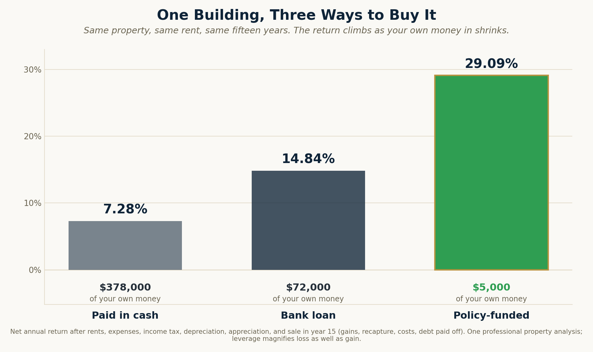
Nothing about the building improved. The rent did not rise, the appreciation did not accelerate, and at the fifteen-year mark the property is worth about $560,868 in all three columns — $360,000 compounded at 3% — for a gain of roughly $200,868 before selling costs, recapture, and tax. The asset performs identically. What changes is the size of the denominator.
A return on invested capital is measured against the money you put in. Scenario 1 measures the property’s own unlevered performance: 7.28% net annualized — a yearly rate across the full fifteen years, not a cumulative total. That is the honest yardstick for the building itself, and it is the rate every other scenario borrows against.
Scenario 2 introduces the first positive spread. The bank’s money costs less than 7.28%, so every borrowed dollar earns more than it costs, and the surplus accrues to the $72,000 that is actually Marcus’s. The unlevered 7.28% becomes 14.84% a year, net, on his own capital.
Scenario 3 introduces the second. The policy loan costs 5.30% — comfortably below the 14.84% the leveraged position is now producing — so a second layer of positive spread stacks on the first, and it accrues to the $5,000 that remains his. The unlevered 7.28% becomes 29.09% a year, net — annualized, not cumulative.
Two layers of borrowing, each costing less than the thing it buys. That is the entire mechanism. There is no third thing happening.
Which is also the warning. Both layers are symmetrical. If the property underperforms its borrowing cost, the same two layers magnify the shortfall in exactly the same proportion — and the buyer with $5,000 in the deal loses it far faster than the buyer with $378,000. Leverage is a multiplier, and it does not read the sign of the number it multiplies.
The 7.28%, 14.84% and 29.09% figures are internal rates of return on the complete fifteen-year after-tax cash-flow stream, produced in a professional real-estate analysis tool. Behind each one the model carries the year-by-year loan amortization and the shifting split between interest and principal; annual depreciation of the improvements and the tax shelter it provides; income tax at 30% on the net rental income after that shelter; fifteen years of 3% compounding on the property value; selling costs at disposition; capital gains at 20% on the appreciation; and depreciation recapture at 25% on everything previously deducted. Scenario 3 additionally carries the policy loan’s 5.30% interest and its repayment schedule.
Could you rebuild the 29.09% from this page alone? No — and I would rather say so than let the page imply otherwise. Reproducing it exactly requires several inputs that belong in a spreadsheet rather than in prose: the note’s interest rate and its thirty-year amortization schedule, the split of the purchase price between land and depreciable improvements, the vacancy assumption, the growth rates applied to rents and to expenses, and the selling costs at disposition. This page gives you every input that drives the conclusion and every output the model produced. It does not give you the model. What it does guarantee is the comparison itself: across all three financing methods, every input is exactly the same — same property, same price, same rents, same expenses, same appreciation, same holding period — and the only variable that changes is the source of the capital. That is what makes it an apples-to-apples comparison rather than three different deals.
That is a limit of the format, not a hiding place — and it has a simple remedy. The analysis was run in the same real-estate calculator I use with clients, and I am glad to open it and walk you through it line by line, on your own numbers, in a single sitting. If a figure in this section does not survive that scrutiny, you should not do business with me. There is no appendix long enough to substitute for that conversation, and I would rather have the conversation.
One more thing, offered because it is the kind of thing a careful reader checks. In Scenario 3, Marcus has $5,000 of his own money in the deal and the property throws off $7,272 a year. If he simply pocketed that cash flow, the first-year cash-on-cash return on his own capital would be 145%. That number is arithmetically correct, and it will not appear anywhere in this paper as a claim. He does not pocket it. It goes to the policy loan, and Section 8.2 explains why that choice is the only one that makes the comparison honest.
Two honest points keep the 29.09% from being a magic trick, and both belong on the page before a skeptic raises them.
8.2 The $0 cash flow is a choice, not a constraint
The property in Scenario 3 still produces the same ~$606 a month it produced in Scenario 2. Marcus elects to route that $606 to repaying the policy loan rather than pocketing it. I show it that way on purpose, because it is the only true apples-to-apples comparison — otherwise Scenario 3 would quietly enjoy both a higher return and free monthly cash flow, which would be stacking two benefits and presenting them as one. Naming it as a choice is what keeps the exhibit clean.
8.3 Repayment rebuilds borrowable liquidity
Every dollar the property sends back to the policy loan does three things at once: it reduces the loan interest; it restores exactly that much borrowing capacity; and the underlying cash value never stopped compounding. Contrast a mortgage paydown, where the equity is locked in the wall until you sell or refinance. Here, the repayment is the liquidity rebuilding. That is the answer to the fair question — “paid back with what, and then what?” The property pays it back, and the capacity returns as it is repaid.
8.4 Now bring the policy back in
The $67,000 that funded the down payment was borrowed against Marcus’s cash value, not withdrawn from it. The money never left the policy. So while that $67,000 was doing its job as a down payment on a property returning 29.09%, it was still a life-insurance asset — compounding, and carrying its death benefit.
The loan is drawn at the end of year six, at 5.30%, and the property repays it. Recall the leveraged owner’s net cash flow from Section 8.1: $606 a month, which is $7,272 a year ($606 × 12). Beginning in year eight, that $7,272 is routed to the policy loan. Marcus’s own premium does not change — it remains $12,000 a year, exactly as before. What changes is the total outlay reaching the policy: $12,000 of his premium plus $7,272 of the property’s rent, or $19,272 a year. The illustration shows that step-up on its ledger, and the rent is where every additional dollar of it comes from.
By year twenty the balance is retired — the final repayment is a partial one, $7,090 rather than $7,272 — and the outlay drops back to Marcus’s $12,000 premium. Through all of it, the policy keeps building.
| Year | Age | Premium | Loan repaid | Total outlay | Loan balance | Net cash value | Net death benefit |
|---|---|---|---|---|---|---|---|
| 6 | 48 | $12,000 | — | $12,000 | — | $74,977 | $411,609 |
| 7 | 49 | $12,000 | — | $12,000 | $70,551 | $19,318 | $367,737 |
| 8 | 50 | $12,000 | $7,272 | $19,272 | $66,633 | $39,016 | $397,198 |
| 10 | 52 | $12,000 | $7,272 | $19,272 | $58,162 | $81,893 | $457,882 |
| 15 | 57 | $12,000 | $7,272 | $19,272 | $32,732 | $216,713 | $629,817 |
| 20 | 62 | $12,000 | $7,090 | $19,090 | $0 | $393,137 | $826,478 |
| 25 | 67 | $12,000 | — | $12,000 | $0 | $581,400 | $1,013,303 |
The year-seven figure looks like a collapse and is not. The freshly drawn loan is netted against the cash value; as the property repays it, the net value climbs back and well past where it started. By age 67 the policy holds $581,400 of cash value and $1,013,303 of net death benefit — while having served as the collateral that turned a $5,000 out-of-pocket commitment into a 29.09% return on a real property. One dollar, two jobs. Both real, both on the illustration.
It is worth being exact here, because the flattering version of this answer is wrong and a careful reader will catch it.
Marcus paid $12,000 a year, exactly as he would have anyway. The tenant retired the policy loan — $94,354 all in with interest — and Marcus never wrote a repayment check. That is the true and useful claim, and it is enough.
What would not be true is to call that $94,354 additional funding of the policy. It is not. Section 12.1 is explicit that a policy loan is not a withdrawal: the money comes from the carrier’s general account against the cash value as collateral, the cash value itself never leaves, and the loan interest is paid to the carrier. Repaying the loan therefore restores the collateral position; it does not add $94,354 of value to the contract.
The illustration proves the point. Left entirely alone, this policy reaches age 67 at $593,235 of cash value and $1,032,395 of net death benefit. Carrying the real-estate loan, it reaches $581,400 and $1,013,303 — about $11,835 less cash value and $19,092 less death benefit. Borrowing costs something, and the ledger shows exactly what.
So the honest accounting of this exhibit is: $11,835 of foregone policy value, in exchange for a rental property that turned $5,000 of out-of-pocket capital into a 29.09% net annualized return, a loan a tenant retired on Marcus’s behalf, and a cash value that compounded uninterrupted throughout. That is a trade worth making on its own terms. It does not need to be described as free.
That sentence is easy to skim past. It is the most consequential one in this section.
A mortgage paydown buries equity in a wall; you cannot spend it again without selling or refinancing. A policy loan repayment restores borrowable capacity the moment it lands. So watch what is actually happening on Marcus’s balance sheet while the tenant works.
| Policy year | Age | First loan still owed | Net cash value | Against the original $67,000 |
|---|---|---|---|---|
| 7 | 49 | $70,551 | $19,318 | Just borrowed |
| 10 | 52 | $58,162 | $81,893 | 1.2× — already restored |
| 13 | 55 | $43,698 | $158,237 | 2.4× — and the first loan is still outstanding |
Three forces compound at once. Marcus’s $12,000 premium keeps arriving. The tenant’s rent keeps retiring the loan. And the underlying cash value — the whole of it, the borrowed portion included — never stopped growing, because nothing was ever withdrawn. By policy year thirteen his net cash value is $158,237: nearly two and a half times the $67,000 he borrowed to buy the building, and the first loan still has $43,698 outstanding against it.
So a question presents itself, and for once it is not rhetorical. Marcus has $158,237 of net cash value, a tenant retiring his first loan on schedule, and twelve working years left. What does he do with the capacity he has rebuilt?
Whatever he does, notice the shape of it. Each deployment brings a cash flow that repays the loan that funded it. Each repayment restores the capacity that funds the next. The premium keeps arriving underneath all of it, and the whole cash value compounds without interruption throughout, because at no point was any of it withdrawn. That is not a higher rate of return. It is the same capital deployed more than once in a lifetime — each deployment acquiring something that pays for itself.
And the next deployment need not be a building. Section 7 argued that opportunities are rarely absent from a person’s life; they are unseen, filtered out before they ever reach conscious attention by a mind that has no capital to act with and no reason to look. Fund the opportunity account, supply the judgment, and what was invisible becomes obvious. What Marcus finds is not something this paper can prescribe, and does not need to. It might be another property. It might be something closer to home.
Follow the cash value while the loan is being repaid, because three engines are pushing it at once and they compound on each other.
| If the first loan is the only one — years 7 to 20 | Amount | Source |
|---|---|---|
| Marcus’s premium | $156,000 | Thirteen years at $12,000 — unchanged from what he was paying anyway |
| The property’s rent | $94,354 | Twelve years at $7,272, plus a final partial payment of $7,090 |
| Credited by the policy | $123,465 | Contractual interest and dividends on the whole balance, net of loan interest |
| Increase in net cash value | $373,819 | From $19,318 in year seven to $393,137 in year twenty |
The third line is the one worth sitting with. The policy credited $123,465 across those thirteen years — net of every dollar of loan interest — because the cash value never stopped compounding on the whole balance while $67,000 of it was out working as a down payment. Marcus’s contribution never rose. The tenant paid the loan. The collateral grew the entire time.
A mortgage paydown buries equity in a wall. A policy loan repayment hands the capital back to you, ready to be used again — and the collateral behind it never stopped growing.
Without the policy, none of this happens the same way. Marcus needs $72,000 of cash for the down payment. He can save it — six years at $12,000 — and then he spends it, and it is gone: no compounding, no death benefit, no capacity restored, nothing standing behind the next opportunity. Or he directs that $12,000 a year into a retirement account, where it grows but cannot be reached without penalty before he is fifty-nine and a half, and cannot be the down payment on anything. Either path forces the same choice: the money grows, or it works. With the policy, Marcus put in $5,000, borrowed the rest against capital that never stopped compounding, and the tenant paid it back. The money bought a building and stayed invested.
Most assets make you choose between growing your money and using it. This one does not.
The table above describes the version of Marcus who stops here — who takes one loan, buys one building, and never borrows again. He does well. By sixty-two the loan is retired, the rent is his to keep, and his net cash value is $393,137.
But that is not the version of Marcus the ledger describes, because the question a rebuilt capacity invites is not whether to use it again. It is what for. And the answer, when it came, was not another building.
8.5 The second deployment — when the opportunity is not a building
Policy year fourteen. Marcus is fifty-six, with twelve working years ahead of him. His net cash value is $158,237. The building’s tenant is still retiring the first loan on schedule, $7,272 a year, without a single dollar from Marcus.
He borrows $100,000 against the policy. Not for a second property.
Suppose he owns a specialty contracting business — the kind a great many readers of this paper own. The $100,000 funds a second crew, a truck and the equipment to put in it, and the marketing to keep both crews busy. Or suppose he owns nothing yet, and this loan starts the business: twelve years before retirement is enough time to build something real, if it is built well. The illustration does not care which. The capital is the same and the ledger is the same.
The expansion produces $10,000 a year of additional net income beginning the following year. That is a 10.0% return on the capital deployed — deliberately modest for a business, and slightly below the 10.9% the building already returns on its own loan. Nothing here depends on the business being extraordinary. It depends on it being competent.
Now two cash flows service two loans. The building sends $7,272. The business sends $10,000. Together they send $17,272 a year, and the total reaching the policy becomes $12,000 of Marcus’s premium plus $17,272 of income the loans themselves created — $29,272.
| Policy year | Age | Premium | Loan repayments | Total outlay | Loan balance | Net cash value | Net death benefit |
|---|---|---|---|---|---|---|---|
| 7 | 49 | $12,000 | — | $12,000 | $70,551 | $19,318 | $367,737 |
| 8 | 50 | $12,000 | $7,272 | $19,272 | $66,633 | $39,016 | $397,198 |
| 13 | 55 | $12,000 | $7,272 | $19,272 | $43,698 | $158,237 | $558,204 |
| 14 | 56 | $12,000 | $7,272 | $19,272 | $143,656 | $80,664 | $487,557 |
| 15 | 57 | $12,000 | $17,272 | $29,272 | $133,083 | $114,955 | $527,296 |
| 20 | 62 | $12,000 | $17,272 | $29,272 | $71,190 | $316,954 | $746,666 |
| 24 | 66 | $12,000 | $17,272 | $29,272 | $8,785 | $523,680 | $953,210 |
| 25 | 67 | $12,000 | $8,785 | $20,785 | $0 | $573,781 | $1,001,012 |
Read the premium column, and then read it again. It is $12,000 in year one and $12,000 in year twenty-five. It never moves. Everything above it was paid by the building and the business the loans bought.
Both loans are retired in policy year twenty-five — the year before Marcus retires. Across those twenty-five years the policy receives $532,409 of total outlay against $300,000 of his premium. The difference, $232,409, retired $167,000 of policy loans and $65,409 of interest on them. Marcus contributed none of it.
One point of precision, since the carrier’s ledger and the plan describe the same money differently. The illustration books those repayments as paid out of pocket, because from the carrier’s side of the transaction that is exactly what they are: a check arrives. In the plan, the money to write the check comes from rent and business income the loans created. Both statements are true. Confusing them is how this category gets itself into trouble.
The illustration routes a flat $7,272 and a flat $10,000 to the loans for as long as they run. In practice both should rise — rents move with inflation, and a healthy business grows — while the bank’s mortgage payment is fixed for thirty years and does not move at all. Holding both flat understates how quickly the loans retire and how much cash flow is free afterward. Nothing in this paper depends on that upside, and none of it is claimed.
Everything has a price, and this one is legible. Set the same contract beside itself — once left alone, once borrowed against twice.
| At age 67 | Policy left alone | Both deployments made |
|---|---|---|
| Net cash value | $593,235 | $573,781 |
| Net death benefit | $1,032,395 | $1,001,012 |
| Annual retirement income | $38,000 | $36,835 |
| He also owns | — | A rental property and a business |
Marcus’s retirement income falls by $1,165 a year — 3.1%. His death benefit falls by $31,383. In exchange, the version of Marcus who borrowed twice arrives at sixty-seven owning a building and a business that the version who left the policy alone does not own at all.
Three percent of his retirement income bought a building and a business.
That is the trade, stated in both directions, with nothing hidden on either side of it. Whether it is a good trade depends entirely on the building and the business — which is to say, on Marcus. The policy did not make the deployment good. It made the deployment possible, and it kept compounding while he made it.
8.6 A note for the reader who knows to ask
This carrier is a Direct Recognition company: while a loan is outstanding, the dividend on the borrowed portion of the cash value is adjusted, which is visible on the illustration in year seven. It is worth understanding and not worth over-reading.
Recognition method is not a free dial you can turn by shopping for a Non-Direct carrier. It is one bundled feature of an entire contract, priced alongside the contractual guarantees, the dividend scale, the loan provisions, and the financial strength of the company — and depending on the rate environment, direct recognition can credit the borrowed portion up rather than down. A Non-Direct carrier recovers the cost of “borrow with no dividend effect” somewhere else in the design.
The honest rule is to weigh the whole contract and the company behind it, never the label on one feature — and never to assume a different carrier would reproduce these cash values while you borrowed against them. With that understood, the figures above are the real, contractual result, with recognition already priced into every one of them.
8.7 The caveat that makes the exhibit trustworthy
The mechanism reliably improves the return on a good property. It does not make a bad property good. The same leverage that turns 7.28% into 29.09% turns a loss into a larger loss. Nothing in this exhibit says “expect 29 percent.” It says: on one representative property, under stated assumptions, coordinating the financing changed the return on the buyer’s own capital by a factor of four — and the capital that made it possible never stopped working.
Which is why Section 7’s weld matters more than this table does. Give a person this mechanism without the judgment to evaluate a property, and you have handed them a faster way to be wrong.
The Number Above the Instrument
9.1 The question, before its name
There is a number that sits beneath everything in this paper, and it is not a policy number.
If the income earner in a household were gone tomorrow, how much would it take to make that family whole? Enough to replace the income the survivors were counting on, for as long as they were counting on it. Enough to clear the debts. Enough to cover the one-time costs nobody budgets for. And enough to leave what the family actually meant to leave.
Answer that, and you have a figure. The figure comes first; the name comes second. The name is Human Life Value — and it is a question about protection and legacy, which makes it a whole-plan number, not something a single policy should decide.
9.2 The calculation
The arithmetic is unglamorous, which is part of why it is trustworthy.
| Component | What it captures |
|---|---|
| Present value of income to replace | The survivors’ future income need, discounted to today |
| Plus outstanding debts | Mortgage, business obligations, anything that does not die with the earner |
| Plus one-time cash needs | Final expenses, education already promised, an emergency runway |
| Less existing assets | What the family already holds and could liquidate |
| Less existing coverage | Group life, individual term, anything already in force |
| = Human Life Value | The family’s human-capital number |
Two disciplines make it honest. The inflation and net-return assumptions default to conservative figures — which makes the computed need larger, not smaller, so the tool never understates a family’s need in order to ease a sale. And the client edits the inputs themselves and watches the number move. They arrive at their own figure rather than receiving one. That is the same posture as the loan-use framework: give the framework, never the prescription.
9.3 The honest number frequently points to term
A system that only ever concludes “buy more of the thing I sell” is not a system. It is a sales pitch with footnotes.
Here is the proof that the analysis follows the math rather than the sale. Run Human Life Value honestly for most working households and the number is large — frequently larger than a cash-efficient whole life policy alone should carry, precisely because that policy is engineered to build cash rather than to maximize early death benefit. Marcus’s policy starts at $251,264 of protection. His household’s honest Human Life Value is almost certainly a multiple of that.
The honest way to fill the gap is frequently term insurance, layered alongside, at a small fraction of the cost. Saying so out loud is not a concession. It is the entire credibility of the approach, and the practitioners in this field worth learning from say the same thing: keeping term in place is, very often, exactly what the number requires.
The instinct to fold Human Life Value into the case for whole life should be resisted, and resisting it makes the number far more powerful. Placed inside the policy discussion, it reads as a way to justify buying more of the policy. Placed above the whole plan, as the honest measure of total protection need, it becomes something better: a figure the family arrives at themselves, which can then be filled by term, by whole life, or by a coordinated mix.
9.4 It gives Continuity its number
Human Life Value is also what turns the legacy claim from an assertion into a figure. “Your family is protected” means nothing until there is a number attached to what protected means. Human Life Value is that number — the destination the self-completing plan funds from the day it is in force. It is what connects the protection conversation, where many families enter, to the capstone the whole system is climbing toward.
The Coordination Payoff Across Phases
Everything so far has described mechanics. This section states what they accomplish when they run together, which is the only claim this paper actually makes.
10.1 In accumulation
The reserve is not idle. Seam One closes: the household’s blended return rises by roughly a point without taking a dollar of new market risk, because the cash that was always going to sit there is now sitting somewhere contractual. And the capital is staged — available on days a bank cannot move, positioned for its highest use rather than leaking into purchases that lose value.
10.2 In distribution — the buffer, and why it must exist before it is needed
Seam Two closes here, and this is where the coordination payoff is largest. It is also the one that cannot be retrofitted.
During accumulation, the order in which returns arrive is irrelevant. Reorder twenty-five annual returns any way you like and the ending balance does not move a dollar, because multiplication is commutative. This is not a rule of thumb; it is arithmetic, and it is why the whole industry is comfortable quoting averages.
The moment withdrawals begin, that indifference disappears, and order becomes the dominant variable. Take the household from Section 2.2 — $1,000,000, drawing $48,000 a year. An ordinary 15% decline leaves $850,000; the year’s income brings it to $802,000; and the portfolio now needs a 24.7% gain simply to return to where it started — and more than that if the next year’s income is drawn before the recovery arrives, while continuing to fund every subsequent year. The shares sold at depressed prices to buy groceries do not come back. They are not a loss on paper. They are a permanent reduction in the base that every future return compounds against.
In the down year itself, both households draw that year's income the same way — from the portfolio — because no one knows in advance how a year will end. The difference appears the following year, once the loss is a fact. A household with only a pile has no second option: next year's income comes out of the portfolio again, selling more shares at the depressed level and locking the damage in. A household with a coordinated system draws the following year's income from a position whose value did not fall — the policy's cash value — and leaves the portfolio untouched to recover on its full balance, returning to portfolio withdrawals once it has. Same market, same returns, same ordinary bad year. One structure has an answer for the year that follows it and the other does not.
You cannot build the second source after the bad year arrives. It exists at the start of the year that follows a loss, or it does not — and whether it exists was decided years earlier, while you were still working.
Which is the whole reason an accumulation-phase decision cannot be graded on an accumulation-phase return. The cash value is not competing with the equity sleeve during Marcus’s working years. It is doing what Sections 5 through 8 describe — earning contractually, standing behind a death benefit, collateralizing a building and a business — and, in addition, quietly becoming the thing his household will reach for on a morning three decades away. The benefit lives in a different phase than the cost. A single-phase return comparison is structurally blind to it, in the same way that weighing a bridge support tells you nothing about whether the bridge stands.
Section 11.4 puts the dollars on the page: Marcus’s contract pays him for twenty-five years and leaves a death benefit, while the market account beside it is exhausted at ninety. It does so without a single policy loan during the pre-retirement years.
How many years of income a household should hold in that second source, when to draw on it, and when to refill it are real questions with real answers, and they are the subject of a separate analysis of the distribution phase. They are not this paper’s subject. What belongs here is narrower and harder to argue with: the capital that makes the option possible has to be accumulated before anyone knows whether it will be needed — by an asset whose accumulation-phase rate of return never told you what it was for.
10.3 In legacy
Marcus’s policy, left simply to run without the real-estate loan, reaches roughly $593,235 of cash value and $1,032,395 of death benefit by age 67. With the loan drawn, deployed into the property, and repaid by that property’s own cash flow, it reaches $581,400 and $1,013,303 — having in the meantime turned $5,000 of his own money into a 29.09% return on a rental he still owns.
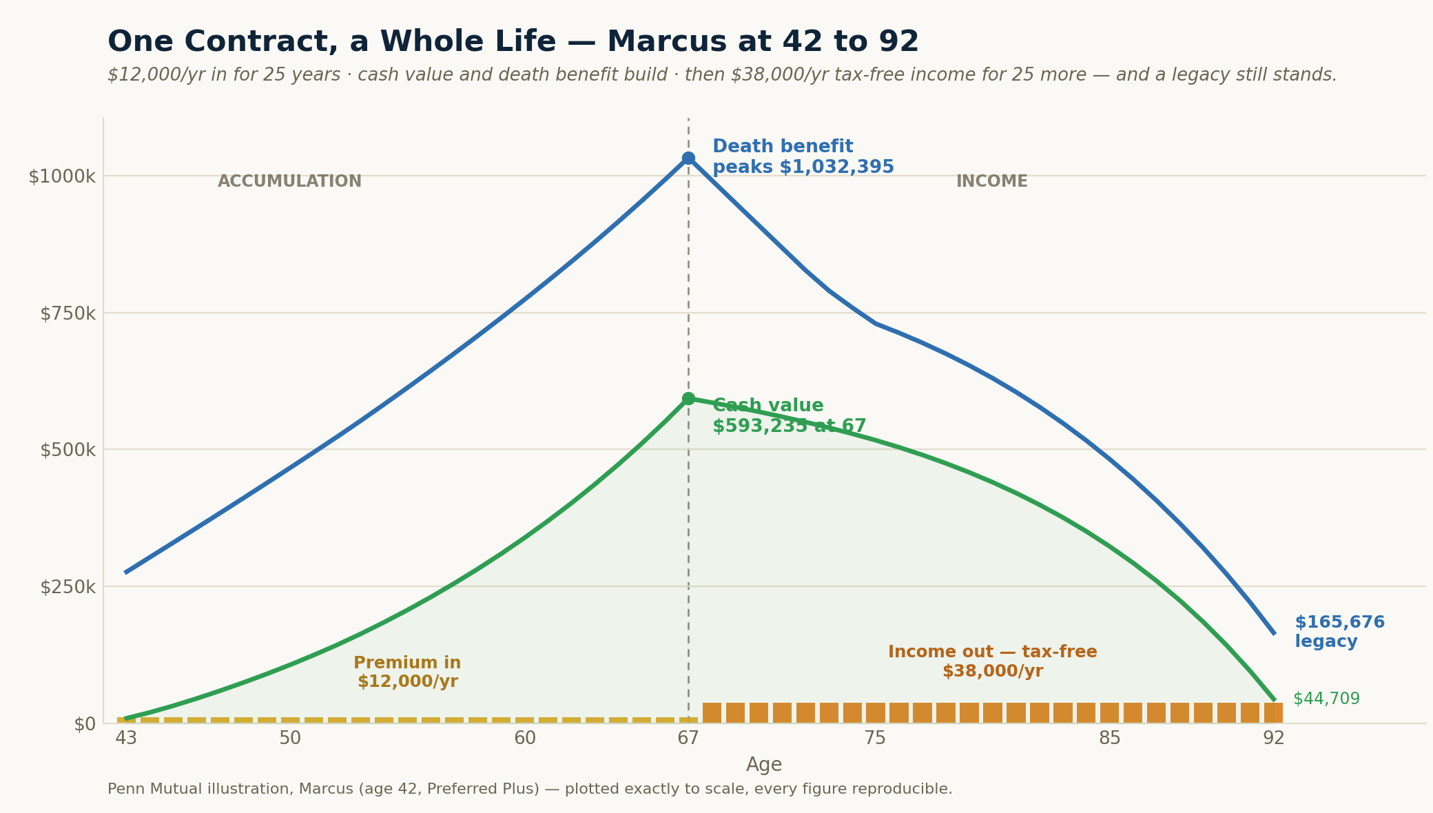
Either way, the death benefit is not an afterthought to the cash value. It is the reason the retiree can spend confidently, because whatever is not spent is replaced. It is what settles any outstanding loan without a schedule. And it is what resets the next generation’s starting line rather than handing them a remainder.
10.4 One asset, several jobs
The reserve that earns while it waits. The account that does not fall when the market does. The capital that keeps compounding while it is being used. The legacy that completes itself the day the contract is in force. Four jobs, one asset, one contract — and the reason a coordinated plan finishes ahead across the whole life of the money, on the result the household actually keeps.
The Net-to-Net Comparison
11.1 This is not a returns contest — and here is the scorecard anyway
Everything above argues that comparing one asset’s return to another’s is the wrong frame. Fine. But a reader is entitled to see the comparison run honestly rather than be told it does not matter, so here it is, with no thumb on the scale.
The illustrated policy produces a Tax-Free internal rate of return of roughly 4.85% on income alone, and about 5.20% including the residual death benefit. Call it 5.00%.
11.2 What the market must actually deliver to match it
The policy’s 5.00% is net of every internal cost and is Tax-Free. To compare fairly, the market portfolio must be asked what compound rate it needs so that, after all four compressions from Section 3, it nets the same outcome. That is an engine solve, not an addition of percentages.
| Investor | Required compound rate | Restated as Average Gross |
|---|---|---|
| Baseline, 1.0% all-in cost | 8.78% | 10.61% |
| Comprehensive managed, 1.5%+ all-in | 9.33% | 11.16% |
The right-hand column adds back the century’s measured volatility gap of 1.83 points, because Average Gross — the arithmetic mean — is how market performance is quoted. The policy needs no such conversion: its growth is contractually positive every year, so there is no gap between its Average Gross and its Actual Net.
If the comparison is instead to a “buy term and invest the difference” plan, the term premium is a real cost and belongs in the market column. A twenty-year term bought at forty-two expires at sixty-two, and across those twenty years the policy’s net death benefit averages $546,000. Replicating it with twenty-year level term at Marcus’s age and best health rating runs $452 a year, which the engine solves to a drag of roughly 0.30 points on the portfolio.
| Buy-term investor | Required compound rate | Restated as Average Gross |
|---|---|---|
| Baseline, 1.0% all-in, plus term | 9.08% | 10.91% |
| Managed, 1.5%+ all-in, plus term | 9.63% | 11.46% |
Now measure those requirements against the actual record of seventy-six rolling quarter-centuries. History delivered less than 10.61% Average Gross in 17 of 76 windows; less than 11.16% in 27 of 76; less than 10.91% in 22 of 76; and less than 11.46% in 33 of 76 — nearly one window in two.
Read that carefully, because it is easy to over-read. It does not say the market usually loses. It says that to merely match what the contract delivers with certainty, the market investor needs to draw a window from history’s deck — and that between roughly one-in-four and one-in-two of the cards on record would have left them short. They cannot choose the card.
11.3 Where the policy actually sits — stated without rounding up
Now the number that most of this category will not print — stated carefully, because the frame matters as much as the figure. Refuse the wrong comparison first: the market's advertised 10.32% is not a number anyone kept, and nothing here concedes it. The honest comparison is to the market's Actual Net — what the four compressions actually left, which across the seventy-six windows had a median of 6.40%, with a quarter of history under 5.45% and a tenth under 4.00%. Against that honest distribution, the policy's illustrated 5.00% Actual Net Return — which assumes the carrier's current dividend scale of 6.00%, itself below 74% of that scale's own thirty-eight-year history — sits, Tax-Free, between the 10th and 25th percentile. It does not approach the median, and the paper does not pretend it does.
Be precise about what that figure is, because the two sides of the comparison are not the same kind of number. The 5.00% is the Actual Net Return this contract projects — net to the policyholder, after policy costs — assuming the carrier’s current 6.00% dividend scale held flat for sixty years, since an illustration is required to assume today’s scale never changes. (The two numbers are distinct: 6.00% is the crediting scale before costs; 5.00% is what the policyholder actually nets, and it is the 5.00% that compares to the market’s net.) The market’s distribution is a century of realized outcomes across every rate environment there has been. One number is pinned to this year. The other roams a hundred. Section 11.6 takes that asymmetry up in full.
Grant that placement — the net one, not the advertised one — and it changes nothing, because the argument was never that the contract out-returns the market on rate. A paper that shaded even the net figure to look better would deserve none of the trust it is asking for.
That is the honest picture, and it is the one worth building on, because the argument was never that the contract out-returns the market. The argument is contractual versus drawn: one outcome is defined in advance, and the other is a card pulled from a deck with a 1.46% floor and a 13.13% ceiling, chosen for you by the year you happened to be born. A household that needs the median to show up is exposed to the tails. A household with a coordinated plan is not.
11.4 Rate is the middle of the story
Section 7 asked what else a dollar of your capital could be doing while you are building. Ask the same question at the other end of the asset’s life and the rate-based objection comes apart entirely.
Two people are sixty-seven. One holds $1,000,000 in a Tax-Deferred account. The other holds Marcus’s policy — $593,235 of cash value, built on $300,000 of premium paid in over twenty-five years.
The first number is not $1,000,000. The tax has not been paid on it. At the 25% combined effective rate used throughout this paper, the spendable balance is $750,000. The policyholder therefore arrives at sixty-seven holding 20.9% less money.
Then the capital is asked to do its final job.
| At age 67 | Tax-deferred account | The policy |
|---|---|---|
| Balance | $1,000,000 | $593,235 |
| Spendable, after tax | $750,000 | $593,235 (Tax-Free) |
| Annual income | $36,000 | $38,000 |
| Payout rate on spendable capital | 4.80% | 6.41% |
| Years of income | 23 full payments, then a partial — exhausted in year 24, at ninety | 25 — ages 68 through 92 |
| Remaining at the end | Nothing | $165,676 death benefit, net of loan |
The holder of the smaller balance draws more income, receives it for two additional years, and still leaves $165,676 behind — after every dollar borrowed along the way has been repaid. Across those twenty-five years he takes $950,000 out of a contract he put $300,000 into, free of income tax, and the contract still pays a death benefit after the final payment. The market account delivers twenty-three full payments and then a partial one, and in its twenty-fourth year — at ninety — there is nothing left to withdraw.
Summary balances conceal the thing that actually decides the outcome, so the account is reproduced on the following page exactly as the cash-flow calculator produces it — every year, every force, nothing removed.
The inputs: present value $1,000,000, current age 67, retirement income $48,000 withdrawn at the beginning of each year, S&P 500 total return, starting year 2001, twenty-five years illustrated. Volatility Drag is captured by using the actual annual returns rather than an average. Activity Drag is applied at 1.50% a year. Tax treatment is Tax-Deferred with terminal taxation at 20% ordinary and 5% state. Fee Drag is 1.00%. Negative balances are not permitted.
The three summary outputs the calculator returns: Average Gross ROR 10.32% · Force drag applied −9.28% · Actual Net IRR 1.04%.
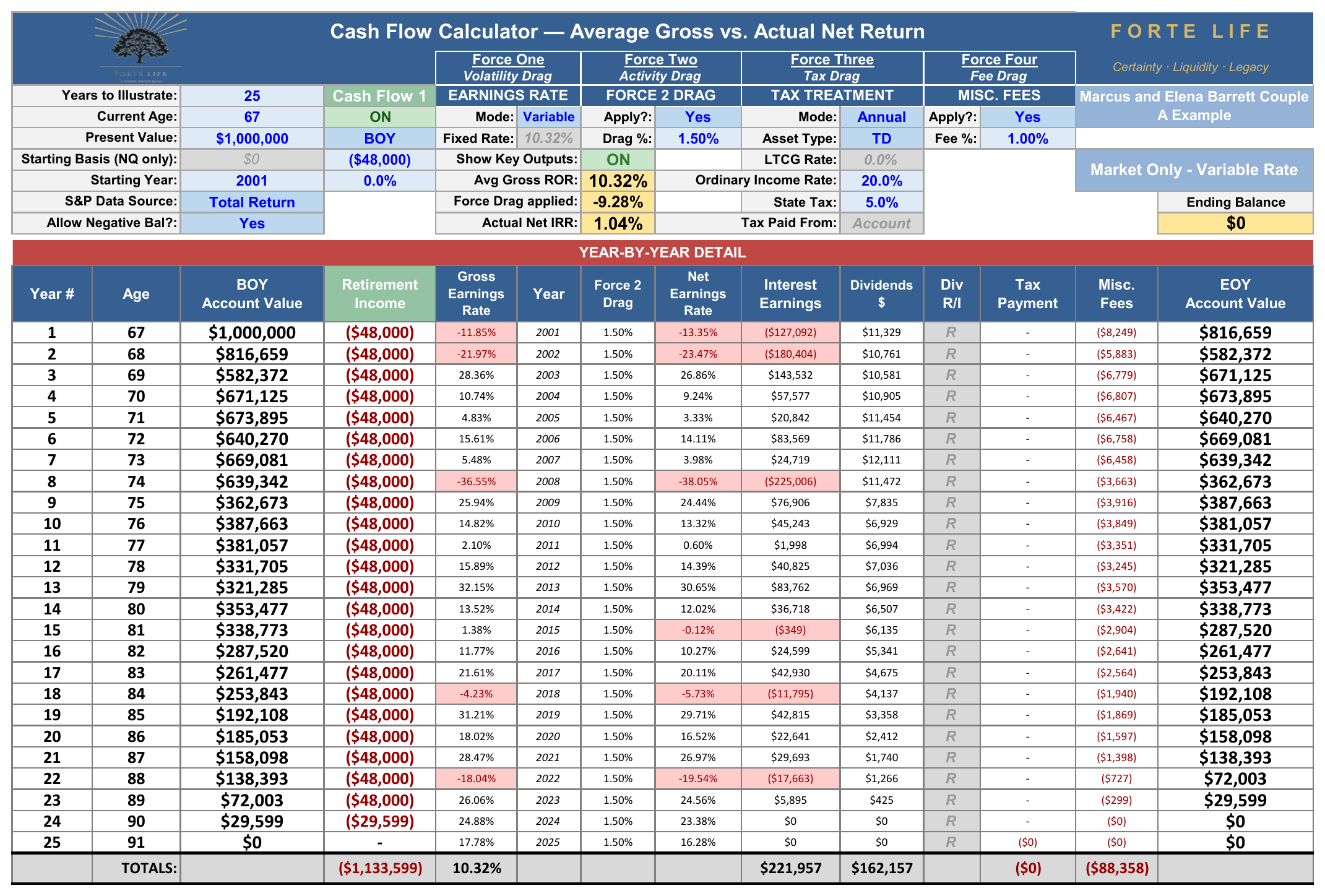
Read the first two rows and the outcome is largely decided. The account earns −11.85% and then −21.97% while $48,000 is leaving it each year, and by the end of year two the balance has fallen to $582,372 — a decline of nearly 42% — from which every remaining year of income must be drawn. The 2008 year takes it from $639,342 to $362,673. After that no run of good years is enough: the account posts gains of 32.15%, 31.21%, 28.47%, and 26.06% along the way and still runs dry, because each of those gains is applied to a balance that withdrawals have already reduced. The same $48,000 that was a 4.8% withdrawal against $1,000,000 becomes a 13.2% withdrawal against $362,673, and no rate of return outruns that for long.
Note the fee column, too. It falls from $8,249 in the first year to $299 in the twenty-third — not because the fee changed, but because the balance it is charged against was disappearing. The total came to $88,358 on an account that ended at zero.
That is the distance between the two figures at the top of the exhibit. The market delivered its advertised 10.32% average across those twenty-five years. The money in this account earned 1.04%.
The market account has to earn a great deal more because it keeps a great deal less. Of every dollar it earns, a share is lost to volatility, a share to the funds and the timing, a share to fees, and a quarter of whatever survives to tax. What is left converts to income at 4.80%, taxable, with a real possibility of running out. Of every dollar the policy credits, all of it stays. It converts to income at 6.41% — nearly a third higher — Tax-Free, without depletion, with a death benefit standing behind it.
Efficiency at the far end removes the need for performance at the near end. The policy never had to stretch, because it never had to make up for what it lost along the way.
A wealth builder’s instinct is to ask what a thing earns, and it is a good instinct. Section 7 argued that the better question is what the capital can do — and aimed it at money about to be deployed. Aim the same question at the asset itself and the answer does not change. What a dollar is worth is not the rate it posts in the middle of its life. It is what it can do across the whole of it: deployed, borrowed against, converted to income, and passed on.
The 29.09% in Section 8 came from capital that was never interrupted. The 6.41% here comes from the same property of the same contract. Uninterrupted capital is the entire argument, and it pays at both ends of the asset’s life. Which is why the percentile in Section 11.3 measures the smaller thing. The market’s advertised average is not what a real investor nets; and even the honest net figure — a median 6.40% across the record — is only a rate, a measure of the smaller thing. Very few windows beat this contract on what the money could actually do on the day it was finally needed.
First, the income is not one mechanism but two. It begins as withdrawals of cost basis — the $300,000 Marcus paid in — and continues as policy loans once that basis is exhausted. It is the combination that keeps all $38,000 of it free of income tax; neither device alone would do it across twenty-five years.
Second, the loan balance that accrues — $1,071,582 by age ninety-two — is settled by the cash value during life and by the death benefit at death. That is precisely why every cash value and death benefit figure in this analysis is a net figure: the outstanding loan is already deducted from it. The $165,676 is what remains after the loan is repaid, not before. Nothing is owed by anyone afterward.
Third, the contract carries an overloan protection rider, exercised in year fifty-one, which prevents the lapse that would otherwise make the accumulated loan balance taxable. Fourth, from year twenty-six through year fifty the premium is met internally through the carrier’s Premium Offset Program — funded by the policy’s own paid-up additions and dividends — rather than out of pocket. Total out-of-pocket outlay stops in year twenty-five, at $300,000.
These are real features of the contract and real conditions of the result. The outcome does not survive if they are ignored, so they are stated here rather than buried in a footnote.
One further condition, from the carrier’s own language: the values above are non-guaranteed and assume the current dividend scale. A change in that scale, in combination with the premium offset, could alter the outcome — including the contract’s tax status. The scale used here sits near the low end of the carrier’s published range since 1989, which is the subject of the next subsection.
Why did the market account run out at all, when its own rate of return was the higher of the two?
Because once withdrawals begin, the order in which returns arrive stops being irrelevant and becomes the dominant variable. During accumulation it does not matter at all — reorder twenty-five annual returns any way you like and the ending balance does not move a dollar, as Section 2.2 noted. In distribution, the same indifference does not hold. The table above shows that mechanism operating on one real sequence; its full treatment — across every sequence, and the planning that answers it — belongs to the analysis of the distribution phase. What belongs here is narrower: the option to be unaffected by it was not created at sixty-seven. It was created decades earlier, by capital that was never interrupted — and by a decision that had nothing to do with which asset posted the better rate.
11.5 The income the other plan never had
Section 11.4 set two retirees side by side and asked what their capital could pay them. It left something out, and leaving it out understated the coordinated plan considerably.
Marcus still owns the building.
Section 8 measured that property across a fifteen-year hold, because a return on invested capital cannot be computed without a sale. But nothing obliges him to sell. Suppose he simply keeps it, and lets rents rise at a modest 2% a year. That growth assumption is introduced here and was not part of the fifteen-year analysis — whose 29.09% depends on a sale that, on this path, never happens. Two different questions, two different assumption sets. They are not added together.
The mortgage payment, meanwhile, does not rise at all. It was fixed on the day it was written. So the gap between what the building collects and what it owes widens every year of Marcus’s life.
One label before the figures, because it matters. What follows is transparent arithmetic on the stated assumptions — 2% annual growth in net operating income against a thirty-year note that never moves — and not an output of the real-estate model. Every number below can be reproduced with a calculator from the two facts above it. That is a different kind of figure from the 29.09% in Section 8, and it is labelled differently on purpose.
| Ownership year | Age | Net rental income | What changed |
|---|---|---|---|
| 1 | 49 | $7,272 | Purchased with $5,000 of his own cash and a $67,000 policy loan |
| 14 | 62 | $14,452 | Policy loan retired — the cash flow is now Marcus’s to keep |
| 20 | 68 | $18,444 | His first year of retirement |
| 30 | 78 | $26,246 | Final mortgage payment |
| 31 | 79 | $44,299 | Mortgage retired — income jumps by $18,053 in a single year |
| 44 | 92 | $57,305 | The final year of his policy income |
Read the last two rows again. Eleven years into retirement the thirty-year note is satisfied, the $17,184 of annual debt service simply stops, and Marcus’s income from this one building rises from $26,246 to $44,299 — an $18,053 raise, at seventy-nine, that arrives because of a decision he made at forty-nine. He did nothing in the intervening years but own the thing and let the tenant pay for it.
Across ages sixty-eight through ninety-two, the property alone pays him $952,144. That is the income stream the market-only plan never created — not because its returns were worse, but because its capital was never available to buy the building in the first place.
Marcus put $5,000 into a property that paid him $952,144 in retirement. A tenant paid for the rest, and the policy never stopped compounding while it happened.
This is the point at which the coordinated plan stops being a matter of degree. Without the policy, Marcus needs $72,000 in cash to buy this building. He can save it — six years of the same $12,000 — and then he spends it, and it is gone. Or he can do what nearly everyone does and route that $12,000 a year into a retirement account, where it compounds respectably and cannot be reached, cannot be borrowed against on his terms, and cannot be the down payment on anything until he is fifty-nine and a half. That is an asset that makes him choose: it grows, or it works.
The policy did not make him choose. The $67,000 bought a building and remained a life-insurance asset, compounding, carrying its death benefit, restoring its own borrowing capacity as the tenant repaid it. One dollar, two jobs — and then, twenty years later, a second income stream in retirement that the other plan has no mechanism to produce.
Section 11.4 compared a policy that was never borrowed against. That is the clean comparison, and it is the right one for measuring a contract against a market account. But it is not the policy Marcus actually owns. His funded the building, and it funded the business. Both loans are on the ledger, and so is their price.
| Ages 68 through 92 | Policy left alone | Both deployments made |
|---|---|---|
| Annual income from the policy | $38,000 | $36,835 |
| Total policy income over 25 years | $950,000 | $920,875 |
| Income from the building | — | $952,144 |
| He also owns | — | A business, and the building itself |
Marcus gave up $29,125 of policy income across a twenty-five-year retirement. The building alone returned $952,144 over the same years — roughly thirty-two dollars back for every dollar of policy income forgone — and the business income is on top of that, unmodelled.
He traded three percent of one income stream for the whole of another.
Two disciplines keep that comparison honest. The $952,144 assumes rents rise 2% a year and Marcus never sells; the 29.09% in Section 8 assumed a sale at year fifteen, and the two figures describe different paths and are never added. And the $36,835 comes from the illustration of the policy with both loans, not from the one Section 11.4 used. Each exhibit names its ledger. None of them are mixed.
What is not in doubt is the direction. The coordinated plan holds a smaller balance at sixty-seven, draws a slightly smaller income from it, and owns two productive assets the other plan has no mechanism to acquire — because its capital was never available without being spent.
11.6 The asymmetry nobody discloses
One further point changes the comparison and is rarely mentioned. Insurance illustrations are required to be conservative: this one projects the current dividend scale — which sits near the low end of the carrier’s published range since 1989, a scale exceeded in roughly three-quarters of that record — unchanged for sixty years. Market projections conventionally use long-run historical averages as a forward assumption.
So the policy is being asked to clear a bar set deliberately low, and the market projection is being asked to clear one set at the optimistic end of its own history. If dividend scales revert toward their long-run average, the policy exceeds its illustration. If forward market returns disappoint — which elevated valuations make a live possibility — the projection does not. The two reference points are not equivalent, and they should not be compared as though they were.
Anticipated Critiques
An analysis of this kind invites scrutiny, and should. What follows steelmans the ten objections a sophisticated reader would raise — a fee-only advisor, a passive-index investor, a CPA, or a practitioner who knows this category well enough to know where it lies. Several of these critiques are aimed at claims commonly made in this instrument’s favor. Those get answered first, because a paper unwilling to correct its own side has no standing to correct anyone else’s.
12.1 “You borrow from yourself and pay the interest to yourself.”
The critique. This is the single most repeated claim in this category’s marketing, and it is what causes informed readers to dismiss the whole subject.
Response. It is mechanically false, and I will not defend it. The carrier lends from its general account and accrues the loan interest to itself. Your cash value is separately, and continuously, earning contractual interest and any declared dividends. The net effect can resemble self-payment; the mechanism is a collateralized loan from a third party. The honest version is stronger anyway: your capital keeps compounding, uninterrupted, while you deploy the carrier’s capital. That is why the phrase throughout this paper is borrow AGAINST, never borrow from.
12.2 “All your money is working from day one.”
The critique. Presentations frequently imply immediate efficiency, or positive loan arbitrage in the early years.
Response. There is none, in any honestly designed policy. Every policy has a capitalization period; first-year accessible cash value runs roughly 70–80% of premium, and Section 4.5 puts the actual year-by-year figures on the page. Anyone promising day-one efficiency is usually selling an oversized policy engineered to flatter year-one numbers at the cost of long-run performance. This is infrastructure. Infrastructure is capitalized before it produces.
12.3 “It replaces your bank, or your 401(k).”
The critique. The absolutist framing — abandon market investing, fire your bank — is what powers the backlash against this entire subject.
Response. It is wrong, and this paper’s architecture rejects it. A coordinated plan requires market-based growth as a component. The instrument completes a plan; it does not replace one. Section 13 states the boundaries explicitly.
12.4 “The average American pays 34 cents of every dollar in interest.”
The critique. This figure headlines a great deal of marketing in this category. It is also the most common factual takedown critics use against it.
Response. It is unsourced and decades old, and it should be retired. Federal Reserve household debt-service data puts required debt payments near ten percent of disposable income — dramatically lower than the legend, and still an enormous sum when compounded across a lifetime of financing. The case stands on the honest number. It does not need the legend, and a body of work that used it would forfeit the right to be believed anywhere else.
12.5 “The loan interest makes it a wash.”
The critique. You borrow at 5.30% against cash value earning around 5%. Net of everything, the arbitrage is illusory.
Response. A policy loan carries a real cost — conceded, and stated in Section 5.3. But the underlying cash value continues to grow during the life of the loan, so the interest is paid on money that is still working, and whether the transaction is worthwhile depends entirely on what the borrowed dollar does. Against a use returning 29.09%, it is not a wash. Against financing a depreciating car you would have bought anyway, the difference is small enough not to matter — which is precisely why Section 7 argues that optimizing the loan rate is optimizing the wrong variable.
12.6 “Direct recognition ruins the strategy.”
The critique. If the carrier reduces the dividend on borrowed cash value, the uninterrupted-compounding claim collapses.
Response. It does not, and the exhibit in Section 8 shows the real, contractual outcome with recognition already priced into every figure. Recognition method is one bundled feature of an entire contract, not a standalone switch you beat by carrier-shopping; a Non-Direct carrier recovers the cost of that feature elsewhere in the design, and depending on the rate environment direct recognition can credit the borrowed portion up rather than down. The disciplined position is to weigh the whole contract and the company behind it, and never to assume a different carrier reproduces these cash values while you borrow against them.
12.7 “It is just collateralized borrowing. A home equity line would do the same thing.”
The critique. The insurance wrapper adds cost and exists only to generate a commission; any equity asset could serve as collateral.
Response. This is the most sophisticated objection in the literature, and the answer is the certainty of access. A home equity line can be frozen or revoked at the lender’s discretion — and was, at scale, in 2008 and 2009. A margin loan can be called precisely when markets fall. A 401(k) loan requires liquidating holdings and is often accelerated on job loss. A policy loan is a contractual right, the collateral is guaranteed by the lender itself, it cannot be marked down, and no repayment schedule can be imposed. The alternatives are cheaper right up until the moment you need them. That is not a commission argument; it is the product.
12.8 “Buy term and invest the difference.”
The critique. Term is dramatically cheaper. Buy it, invest the savings, and finish ahead.
Response. Three separate problems. First, the term premium is a real cost that belongs in the market column — loaded in, the buy-term investor must see an Average Gross of 10.91% sustained for decades to match the contract, and history delivered less than that in 22 of 76 windows. Second, the twenty-year term purchased at 42 expires at 62, five years from retirement. The $546,000 of coverage that cost $452 a year at forty-two costs $3,497 a year at sixty-two — nearly eight times as much — and thirty-year term is not offered at that age at all. Both figures assume the very best health rating, which is a far harder assumption at sixty-two than at forty-two; for some buyers, replacement is not available at any price. Third, and most important, the term-plus-market plan has no answer for Seam Two: the entire retirement portfolio is market-correlated, so there is nothing to draw from in a bad year. And as Section 9 showed, term is frequently exactly right for the protection gap. This was never either/or. A coordinated plan often uses both.
12.9 “Most of these policies are surrendered. Yours will be too.”
The critique. Industry data suggests a large share of whole life policies lapse within ten to twenty-five years. The illustrated outcome assumes a discipline most people do not have.
Response. The aggregate data describes a different instrument: policies sold for death benefit rather than accumulation, without paid-up-additions optimization, to buyers who could not afford the premium or were never taught what they bought. It is a fair indictment of the industry’s execution and a poor description of this design. Two structural answers exist. Once the policy reaches break-even — year five here — it can elect a premium offset arrangement, under which the contract funds its own base premium internally from existing paid-up additions while dividends continue purchasing new ones. The obligation becomes a completed commitment of five to seven years rather than a decision repeated for fifty. That removes the behavioral decision points, which is more than any market account can say.
12.10 “I am too old for this to work,” and “I don’t have a high-return deal.”
The critique. The capitalization period makes it useless for someone within a decade of retirement, and the Category 3 argument only works for people with access to good deals.
Response. Two answers, and neither requires stretching. On age: the twenty-five-year example in this paper is an example, not a requirement. The same policy under a premium offset arrangement, funded for seven years rather than twenty-five, remains in force, continues to grow, and delivers a comparable internal return per dollar contributed — the absolute dollars change, the structure does not. On deals: if there is no high-return deployment, the highest use of that capital is the conservative one — the reserve, the buffer, the cost-of-money saving — and the coordinated plan still wins on the three seams alone. The mechanism improves a good opportunity when you have one. It never requires one in order to be worth holding.
12.11 “I hold Roth dollars, so the tax force does not apply to me.”
The critique. The four forces model a Tax-Deferred account and a terminal tax. A Roth holder pays no tax on the way out, so the third force is neutralized and the comparison overstates what the market actually loses.
Response. Narrowly true, and it changes less than it appears. A Roth holder does not escape the tax — they pre-paid it, on contributions, at today’s rates, and accepted the constraints that come with it: annual contribution caps, income phase-outs that bar many high earners from contributing directly, and a Roth 401(k) option only widely available since the mid-2000s, which is why the great majority of existing retirement balances are still pre-tax. More to the point, a Roth neutralizes one force. The Roth investor still meets volatility and activity in full, still faces sequence-of-returns risk in distribution, and still holds a position that falls when the market falls. Where a reader holds Roth dollars, the tax leg of this comparison narrows accordingly; the other three forces, and the structural case, stand unchanged. The companion Accumulation analysis treats this at length.
What This Analysis Is Not Arguing
To prevent misreading, the boundaries stated plainly.
- It is not arguing that the policy wins a rate contest against the market’s advertised return. That number is not what a real investor keeps; the honest, net comparison is in Section 11.3, stated with the percentile attached and the two-sided asymmetry made explicit.
- It is not arguing against low-cost index investing. For the growth portion of a portfolio, disciplined passive equity investing is mathematically sound and belongs in the plan.
- It is not arguing against paying for advice. Good advice earns its fee many times over. The argument in Section 3 is not that the fee is too high; it is that it should be visible, in dollars, over a lifetime, so the decision belongs to the person paying it.
- It is not arguing that anyone should liquidate existing investments to fund premium. The coordination question is about where new capital goes and where reserves live — not about dismantling what is working.
- It is not arguing that this instrument suits everyone. Households without a stable funding horizon, without insurability, or with already-adequate guaranteed income may not need it, and Section 9’s honest protection number frequently points to term instead.
- It is arguing that coordination is universal, that the seams are real and measurable, and that one properly structured contract can close several of them at once — for the households where it fits.
The Plan That Finishes Itself
Every section of this paper has been about living mechanics — certainty, control, compounding, the highest use of capital. This is where they add up.
Legacy here is not a separate product you buy. It is what the disciplines become when they are run well across time. It is the roof on the walls, not a fourth wall.
So return to the two families from the opening. Every ordinary way of building wealth depends on a clock no one controls: you have to live long enough to finish funding it, and long enough for it to grow. Stop early, and your family inherits the half-built version. This is the one that finishes itself. From the day it is in force, the destination is funded — whether the parent passes tonight or in fifty years. The single event that breaks every other plan is the event this one is built to complete.
The honest boundary, drawn here rather than left for a skeptic: the legacy half of this plan completes the day the contract is in force. The banking half — the cash value you borrow against — does not. It capitalizes over years, with real early limits, exactly as Section 4.5 showed. Legacy completes immediately; the bank matures. Both are true, and saying both is what lets the first claim stand.
The head start is not a pile of cash to start over with. It is a place near the top of the climb the other family is still making.
Four generations on, the first family is back at the bottom of the hill. The second family began this generation where the first is still trying to arrive. Same income. Same market. Same returns. One of them simply never had to start over, and never had to hope the timing worked out.
You do not have to start anything or join anything to live in the second version. It is not a community with a shared rule. It is one household that refused to leave its reserves idle, refused to be forced to sell at the bottom, and refused to let the plan depend on living long enough.
Which returns us to where this began. This asset is never where a plan starts — it is where an honest analysis often arrives. When it leads here, everything in this paper is the reason why. When it does not, the plan is coordinated anyway, which was the whole point.
❦
Methodology and Disclosures
All market figures are measurements of actual S&P 500 total returns, not projections. The century basis is 1926–2025 (arithmetic mean 12.11%, compound 10.28%, measured volatility gap 1.83 points). The primary worked window is 2001–2025 (arithmetic mean 10.32%; twenty of twenty-five years positive; positive years averaging 17.5%). Rolling-window analysis covers all seventy-six overlapping twenty-five-year windows in the century. All balances assume $100,000 initial, a Tax-Deferred account, a 25% combined effective terminal tax rate, a 1.0% all-in annual cost, and a 1.5% annual activity adjustment. Every figure is an output of a single cash-flow engine; none is scaled or estimated.
The 1.5% figure is anchored on the structural component rather than the behavioral one. Over the twenty years through 2024, roughly 92% of active large-cap funds trailed the S&P 500 (SPIVA U.S. Year-End 2024), and roughly 46% of U.S. fund assets remain actively managed. The behavior gap — the shortfall between investor returns and the returns of the funds they hold — is measured at approximately 1.2 points annually (Morningstar, Mind the Gap 2025) and is the smaller and more contested of the two legs; peer-reviewed work in the Financial Analysts Journal argues it is substantially a measurement artifact. The 1.5% assumption does not depend on it. Neither component is presented as investor failure; the larger has nothing to do with the investor.
The 1.0% all-in figure comprises the advisory layer plus embedded costs — fund expense ratios, trading costs, revenue sharing and platform fees, and cash drag. It sits at or below what most advised investors pay once every layer is counted, which means the analysis understates rather than overstates the drag. No fabricated all-in figure is printed anywhere in this paper.
This analysis draws on three separate illustrations of the same contract, and never mixes figures across them. The first shows the policy with no loans taken. The second shows it with the $67,000 real-estate loan. The third shows it with both the real-estate loan and the $100,000 business loan. Every exhibit states which ledger it uses. Years one through thirteen are identical across all three.
All policy values are drawn from a single carrier illustration for a male, age 42, Preferred Plus Non-Tobacco, funding $12,000 annually into a properly structured Accumulation Whole Life contract with maximum paid-up additions, designed as a Non-MEC. Both the base ledger and the with-loan ledger are actual illustration outputs at the current dividend scale. The carrier is a Direct Recognition company, and every with-loan figure reflects that treatment. Dividends and non-guaranteed values are not guaranteed; actual results will differ. Guarantees rest on the claims-paying ability of the issuing insurer.
The three purchase scenarios reflect one representative property analysis under the assumptions stated in Section 8.1, produced in a professional real-estate analysis tool. They are a single worked example, not a prediction, not a typical result, and not an expectation. Leverage magnifies losses as well as gains.
The insurance-puzzle result referenced in Section 5.1 appears in a 2023 editorial in the Annals of Actuarial Science recounting a question posed by Kenneth Arrow. The underlying mathematics — the divergence of arithmetic and geometric growth, and time-average optimization — predates and is independent of any contemporary research program built around it. Household debt-service figures are from Federal Reserve data. Active-manager underperformance figures are from standard industry persistence scorecards. Behavior-gap figures are from published investor-return studies. Dividend histories are carrier-published.
This analysis is provided for educational and planning purposes only and is not tax, legal, or investment advice. Nate Butler is a Retirement Income Specialist, not a financial planner or investment adviser. Policy values and dividends shown are drawn from a specific carrier illustration; non-guaranteed values are not guaranteed and actual results will differ. Loan provisions, recognition method, and availability vary by contract and carrier. Real-estate figures reflect one representative analysis under stated assumptions and are not a prediction. Properly structured whole life insurance is one instrument within a coordinated plan and is not suitable for everyone. Any strategy should be evaluated against your own circumstances with appropriate professional guidance.
FORTE LIFE · CERTAINTY · LIQUIDITY · LEGACY · 1
Where to Begin
If any of this landed, it is probably because you recognized your own plan somewhere in it — good pieces, assembled by different people at different times, never quite coordinated into one system. That is the common case, and it is a fixable one.
The clearest place to start is a Capital Coordination Session — a focused look at how your money is actually put together: whether your accumulation, your income, your taxes, and your legacy are working as one system, or just sitting side by side. You get something of value whether or not you buy anything — you leave knowing where the seams are. What it produces is a coordinated Retirement Income Plan — principles first, then strategy, then whatever instruments the plan actually calls for, with one person designing for the total. The Banking Concept plan is a module inside that plan, not a separate product.