The Order of Things
A Rigorous Analysis of Sequence Risk, the Distribution-Phase Tax Machine, and the Two Systems That Change the Answer
Distribution series · The Order of Things · the Whitepaper — the complete reference, one of four layers.
The Reversalthe Half of the Root That Distribution Owns
All three Forte Life papers — the Accumulation analysis, the Living Asset Strategy, and this one — rest on a single premise, worth stating plainly here so that a reader who has seen one of the others feels corroboration rather than a seam, and a reader who has seen none can still follow from here. You live forward through uncertainty. The future is not a point but a range, uncertain in two dimensions at once — how much the money will earn, and when it will be needed — and the ordinary plan quietly treats both as fixed. You already act on this: every prudent portfolio holds bonds, not because bonds out-earn stocks but to compress the range, trading some average for reliability. And every dollar you own makes the same three-way trade — Growth, Safety, Access: pick two, give up the third. That much the whole body of work shares.
The three papers then divide that premise cleanly. The Accumulation analysis owns the first dimension — how much, the gap between the return the market advertises and the return a saver actually keeps. The Living Asset Strategy owns the instrument that lets a single dollar hold all three of Growth, Safety, and Access at once. This paper owns the second dimension — when — and in the distribution phase that dimension stops being a background condition and becomes the entire game. You do not need to have read the other two: where this paper leans on a result from one of them, it says so and points to where it is established here.
Here is why, stated as plainly as it can be. While you are saving, when a good or bad year arrives does not matter. The dollars stay in the account and ride the recovery, so the order of returns is genuinely irrelevant to where you end up — a fact Section 3 re-proves here in a single paragraph, because it is the hinge the whole argument turns on. The day you begin drawing income, that protection expires. Now every bad year arrives while money is being removed, and the dollars removed at the bottom are gone before the recovery can reach them. The same range of futures that was survivable while building becomes decisive while spending. Time, which was your ally, becomes your constraint.
Every mountaineer knows what the arithmetic just said: the summit is only half the climb, and not the dangerous half. The descent is where the accidents cluster — the legs are tired, the light is going, the margin is spent, and gravity, which fought you the whole way up, is now at your back and pulling. Accumulation is the ascent; distribution is the descent — the same mountain, but the half where a misstep actually costs you. And the descent asks for different muscles, and different tools, than the climb: you brace where you used to drive, and lean on holds and ropes you never needed on the way up. A plan built entirely for the ascent and handed to you unchanged is not a plan for the descent at all — and the descent is the half this paper is about.
So the objective is unchanged — keep a family's resources useful across the whole range of futures — but the phase has changed what "useful" requires. In accumulation it meant growth that survived the four forces of return drag named in Section 2. In distribution it means income that survives the order the market delivers, whatever order that turns out to be. Rate is an input to that. In the distribution phase it is not even the dominant input. The order is. The rest of this paper is the proof — and it begins, as the honest version always does, not with the frightening number but with the ordinary arithmetic that makes the number inescapable.
The Honest BenchmarkWhat a Saver Actually Kept
Before measuring what a retiree keeps, the thing being measured against has to be honest. This section states that benchmark self-contained — everything needed is on this page — and points to where the full derivation lives, so a reader who has never opened the companion Accumulation paper can still follow every step from here.
The market advertises an average. The advertised long-run figure is "10 to 12 percent," and across the specific quarter-century this paper works in — 2001 through 2025 — the S&P 500's arithmetic mean was 10.32%. That number is real, and it is not the number an investor keeps. Four forces stand between the advertised average and the compounded result, and each is measured in full in the companion Accumulation series (subtitle The Actual Net Return): volatility drag (the arithmetic mean of a jagged series always exceeds the rate it actually compounds at), activity drag (most money sits in actively managed funds, and roughly nine in ten of them trail the index they are measured against, before the investor does a single thing), tax drag (in a tax-deferred account the entire balance, not just the gains, comes out as ordinary income), and fee drag (a one-percent all-in cost compounds into slightly more than a point of lost return). Named once, handed back — the derivation lives there, and this paper does not re-run it.
What the four forces leave is the honest benchmark. A saver holding an ordinary advised portfolio through 2001–2025, in a tax-deferred account, kept a compound 4.93% — the advertised 10.32% compressed by more than half. And 2001–2025 was not an unkind draw: across every one of the last century's seventy-six rolling twenty-five-year windows, the median Actual Net a saver kept was 6.40%, with a quarter of history under 5.45%. So the honest planning number — the floor this paper builds on — is the market's Actual Net, a median 6.40% and 4.93% in the specific window worked here, never the advertised average. (The tax-deferred convention throughout — a 25% terminal rate, 20% federal plus 5% state — is likewise established in that companion analysis; this paper adopts it.)
Hold those two numbers next to the advertised one, because the whole of what follows lives in the distance between them and one number still to come. The index made 10.32%. The saver kept 4.93%. That gap is the companion Accumulation paper's central finding, carried in full there and summarized here — and it is already a hard truth.
But it is a truth about a saver — someone whose dollars stayed in the account and compounded. It is not the number a retiree keeps, because a retiree is not compounding a balance; they are drawing one down, in an order they do not choose. The day the withdrawals begin, a fifth thing takes over that the four forces never accounted for, and it compresses the number again — not by a little. The saver's 4.93% is the floor. The retiree's number is below it, and the next two sections build the reason before they state the figure, because the figure is the single most dismissible fact in this entire paper and it has to be earned.
The Ordinary Yearthe Mechanism, Before Any Number
The case for sequence risk is usually made with a crash, and it should not be, for two reasons: a catastrophe lets the reader escape into "that won't happen to me," and — more damning — it is not what does the damage. An ordinary year does. So before any number about retirees appears in this paper, here is the mechanism, in arithmetic no one can reject, with no product anywhere in sight.
Start with the fact that governs the whole saving phase — the one Section 2's benchmark rests on — re-proven here in one paragraph because everything turns on it. Take $100,000 and three returns — up 25%, down 10%, up 15%. In that order the result is $129,375. Reverse it to up 15%, down 10%, up 25% and the result is $129,375. In any order it is $129,375, because the ending balance is the product of the annual factors and multiplication is commutative. That is why, while you are saving, the order of returns cannot hurt you, and why the industry is comfortable quoting averages to savers.
Now start withdrawing, and watch the symmetry break. Same $100,000, same three returns, but take $10,000 out at the start of each year before that year's return applies. In the original order the account ends at $94,587; reversed, it ends at $92,687. Identical returns, identical withdrawals, different endings — and the only thing that changed was the order. Over three years the gap is small. Over a thirty-year retirement, compounded, it is the difference between a plan that finishes comfortably and one that fails.
Then see it at the scale of a real retirement, still with no product in the room. A retiree draws $48,000 from a $1,000,000 portfolio — a 4.8% withdrawal, the figure most planners call prudent — and meets not a crash but an ordinary 15% decline, the kind the market delivers roughly one year in four:
The $1,000,000 falls 15%, to $850,000.
The year's $48,000 of income still comes out, leaving $802,000.
To climb back to where it started, that $802,000 must now gain 24.7% — not the 15% it lost.
Read the last line slowly, because it is the whole mechanism in miniature. An ordinary down year already demands a 24.7% rebound to return to even — and it is worse if the next year's income is drawn before the recovery arrives, which of course it is, because the retiree still has to eat. Nothing improbable happened. This is a normal year doing permanent damage, because the shares sold at a discount to fund living expenses are not there when the market climbs back. The portfolio is structurally smaller for every year that follows. The market did not have to misbehave. It only had to deliver an ordinary loss while money was being drawn — which it does, to everyone, eventually. That arithmetic is the engine. The next section turns it on for a full twenty-five years and lets it produce the number.
The Retiree's NumberEarning the 1.04%
Now the number, and a warning about it first, because it is the most powerful and the most dismissible fact in this entire paper. When you read that a retiree drawing income through the market of 2001–2025 kept a compound 1.04%, every instinct will tell you the claim is wrong — that no one who lived through a market averaging over ten percent could possibly have kept one. That instinct is correct about the market and wrong about the retiree, and the gap between those two things is the entire point.
So let me agree with you before I ask you to believe anything. If you are thinking "the market can't have been that bad" — you are right. It wasn't. Across those twenty-five years the S&P 500 averaged 10.32%. Twenty of the twenty-five years were positive. The winning years averaged more than 17% apiece. By every ordinary measure it was a good quarter-century to have money in the market. That is not the counter-argument to what follows. It is the trap. The damage was never in the market's average. It was in the order — the arithmetic you already accepted in Section 3, now run for a full retirement.
Watch the same twenty-five years produce three different numbers, one staircase step at a time:
The index made 10.32% — the arithmetic average, the number on the brochure.
A saver kept 4.93% — that average, compressed by the four forces of return drag named in Section 2. Believable, and already documented.
A retiree drawing income kept 1.04% — that saver's return, compressed again by sequence risk, because this retiree was not holding the market. They were spending it down, in the order it happened to arrive.
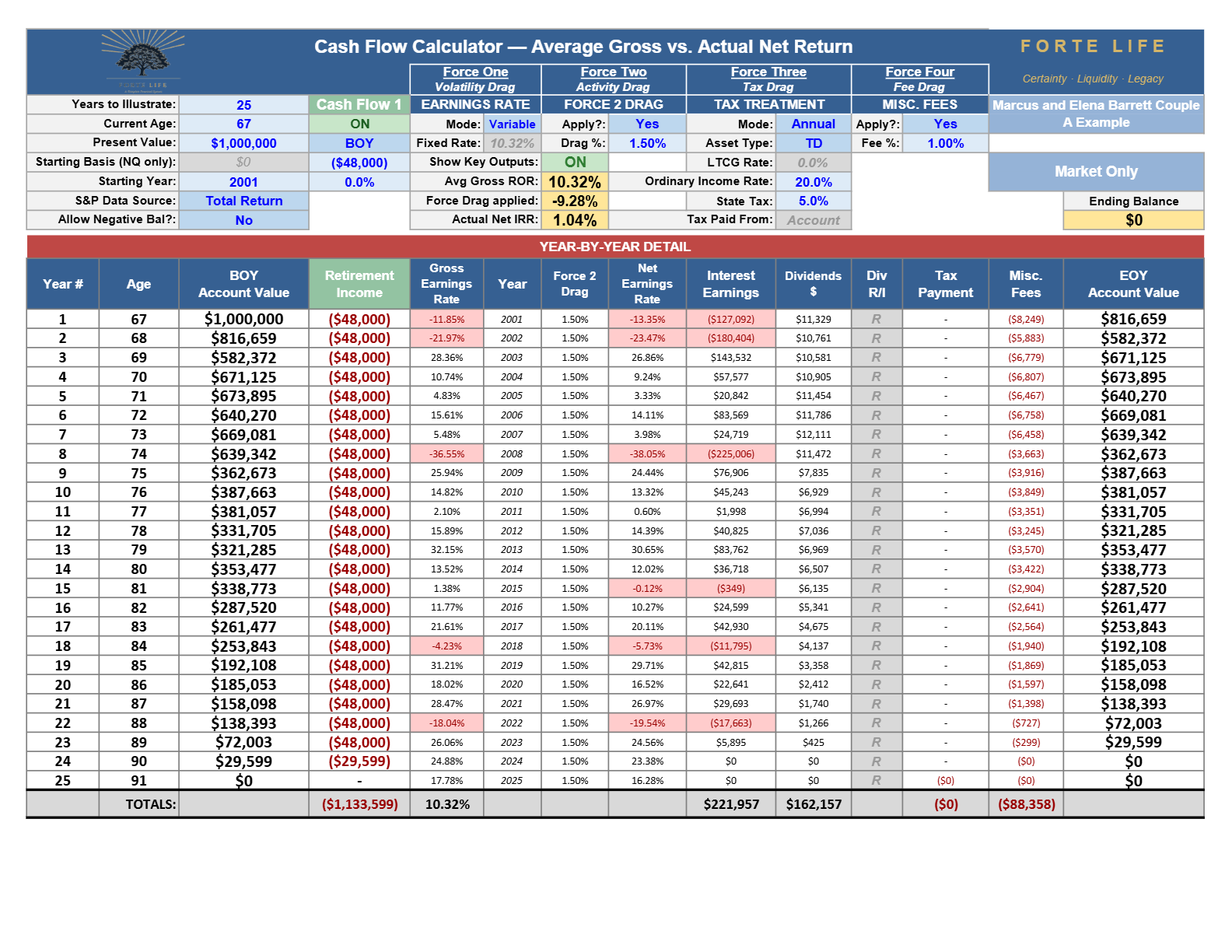
Each step is believable on its own. The endpoint is inescapable because each step before it was. And it is not a rhetorical figure — it is the actual output of the Cash Flow Calculator, run on the real sequence, which you can reproduce on any calculator from the market's own published returns.
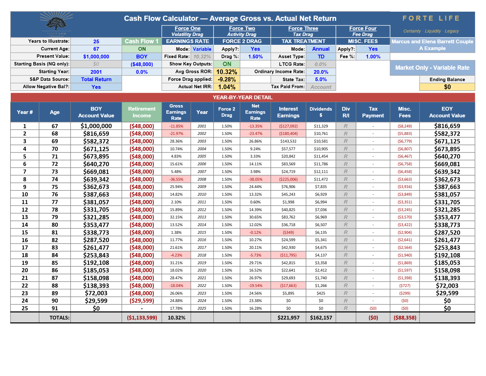
CF Calc: Scenario A (Conventional, market-only). Present value $1,000,000 · age 67 · income −$48,000/yr drawn at beginning of year · S&P 500 total return, 2001–2025 · Volatility Drag via actual annual returns · Activity Drag 1.50% · tax-deferred, 25% terminal (20% federal + 5% state) · Fee Drag 1.00% · negative balances not permitted. The exhibit, rendered. Below is that exported run as its own four-force grid — the authoritative CF-calc output, not a retyped summary. Read the Gross rate column against the Net rate beside it (every year is the gross less the 1.50% Activity Drag), and watch the EOY balance fall as the fixed $48,000 is drawn through it. The account is floored at zero — it stops paying the year it can no longer fund the draw. No CF Calc figure is retyped into a hand-built summary; each is shown as its exported exhibit.
The actual Forte Life Cash Flow Calculator export, year by year, with all four forces applied — never retyped.
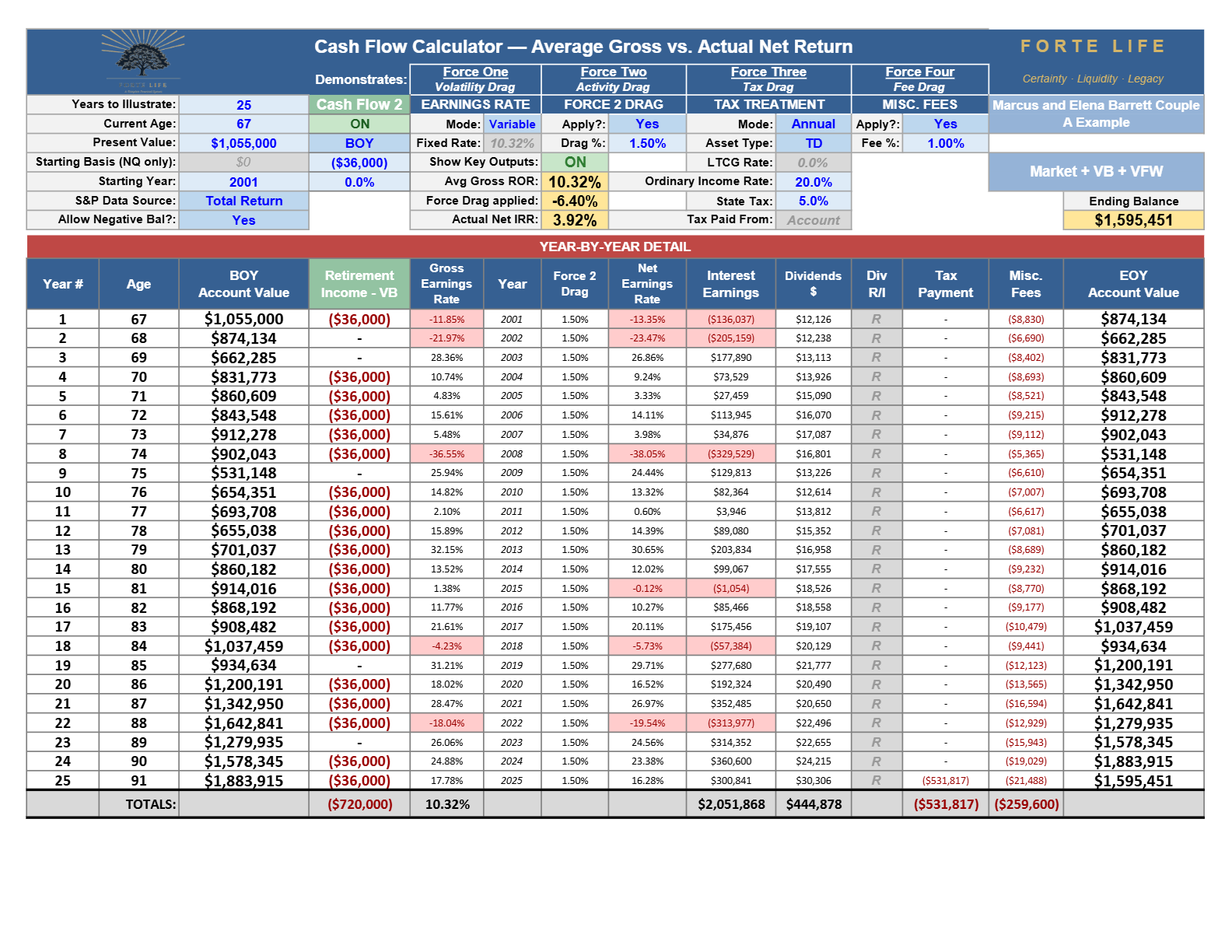
The actual Forte Life Cash Flow Calculator export, year by year, with all four forces applied — never retyped.
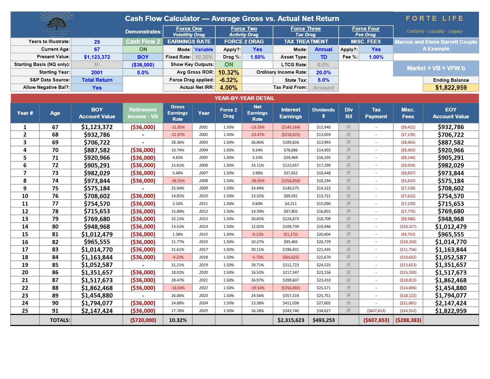
The actual Forte Life Cash Flow Calculator export, year by year, with all four forces applied — never retyped.
Authoritative CF-calc export (S&P 500 total return, 2001–2025), rendered as a grid — the four forces working line by line. Summary outputs: Average Gross ROR 10.32% · total force drag −9.28% · Actual Net IRR 1.04% · ending balance $0. Twenty-three full $48,000 payments (ages 67–89), a final partial payment of $29,599 in year 24 (age 90), $1,133,599 drawn in total, $88,358 paid in fees — on an account that ended at zero.
Do not read that exhibit as a summary; read it as the mechanism caught in the act. The four forces work line by line, every year — the reader can watch 10.32% become 1.04% — and two rows decide the outcome before the story is a third told. By the end of the second year the balance has fallen by nearly 42%, and every remaining year of income must be drawn from that reduced base. Then the part that breaks the disbelief for good: this was not a weak market that simply failed to deliver. Along the way the account posts single-year gains of more than 32%, more than 31%, more than 28%, more than 26% — four separate years better than a quarter — and it still runs dry, because each of those gains applies to a balance that withdrawals had already shrunk. The same $48,000 that was a 4.8% draw against $1,000,000 had become a 13.2% draw against a post-2008 balance of $362,673. No rate of return outruns that for long.
State the contrast the way it should be carried, because the hook is never the raw "one percent." The market delivered its advertised 10.32% average. The money in this account kept 1.04%. Same market, same twenty-five years. That distance is not the four forces of Section 2 — it is a fifth and separate thing. The forces compress every dollar the market earns; sequence risk decides whether the dollars that remain survive being spent in the wrong order. And it cannot be modeled away with an average: at any constant return above 4.8%, a $1,000,000 account drawing $48,000 never depletes. The depletion is purely a sequence effect. That is the proof, and it is why this exhibit — not any argument about products — is the foundation of everything that follows.
One more thing the exhibit cannot show on its own, and it is the reason this has to be understood before retirement rather than during. Sequence risk is invisible in year one. The account that will fail at ninety looks, in its first year, exactly like the account that will thrive — same balance, same withdrawal, same statement. By the time the failure is visible on a statement, the shares that would have carried the recovery have already been sold to pay for groceries. The damage is done in the early years and only seen in the late ones. A risk you can only recognize once it is too late to fix is a risk you have to plan around in advance.
It Was Not the Windowand It Was Not the Model
A fair reader raises the obvious objection here, and it deserves the whole record as an answer, not a sentence. You chose 2001. You rigged the window. If 2001–2025 were a uniquely cruel starting point, the 1.04% would be an anecdote, and an anecdote proves nothing. So the honest move is to stop choosing windows and let the record choose them.
5.1 The record of start-years
Run the same household — $1,000,000, $48,000 a year, the four forces — from every notorious retiree starting point the last century offers, and then run each one again with the Firewall in place. The starting points are exactly the ones a retiree fears: 2000, into the dot-com collapse; 2007, into the financial crisis; 1929, into the Depression; 1973, into the oil shock and the stagflation that followed; and 1966, into the long secular bear that opened the stagflation era and ground on for sixteen years. Each front-loads severe losses — or, in 1966's case, a lost decade and a half of real returns — onto the first drawing years, which is the condition sequence risk feeds on.
CF Calc: the market-only plan and the Firewall plan across six retiree start-years. $1,000,000 · −$48,000/yr · four forces as in 4·A, run for the 2000, 2001, 2007, 1929, 1973, and 1966 start-years, each in a market-only version and a Firewall version (the same $648,649 rolled to a joint lifetime income annuity, remainder invested). The runs, rendered. Each start-year appears below as its exported four-force grid — the market-only plan first, then the same household with the Firewall in place. The failure years are floored at zero (income stops the year the account can no longer fund the draw); the survivor years run the full twenty-five. In every pair, read the market-only EOY balance against the Firewall remainder's.
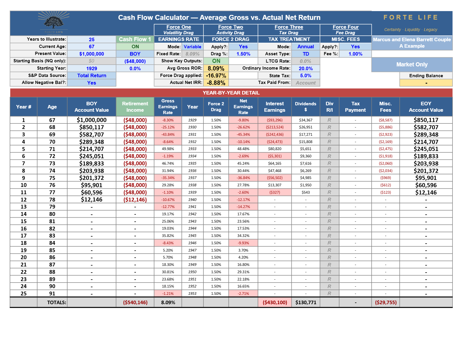
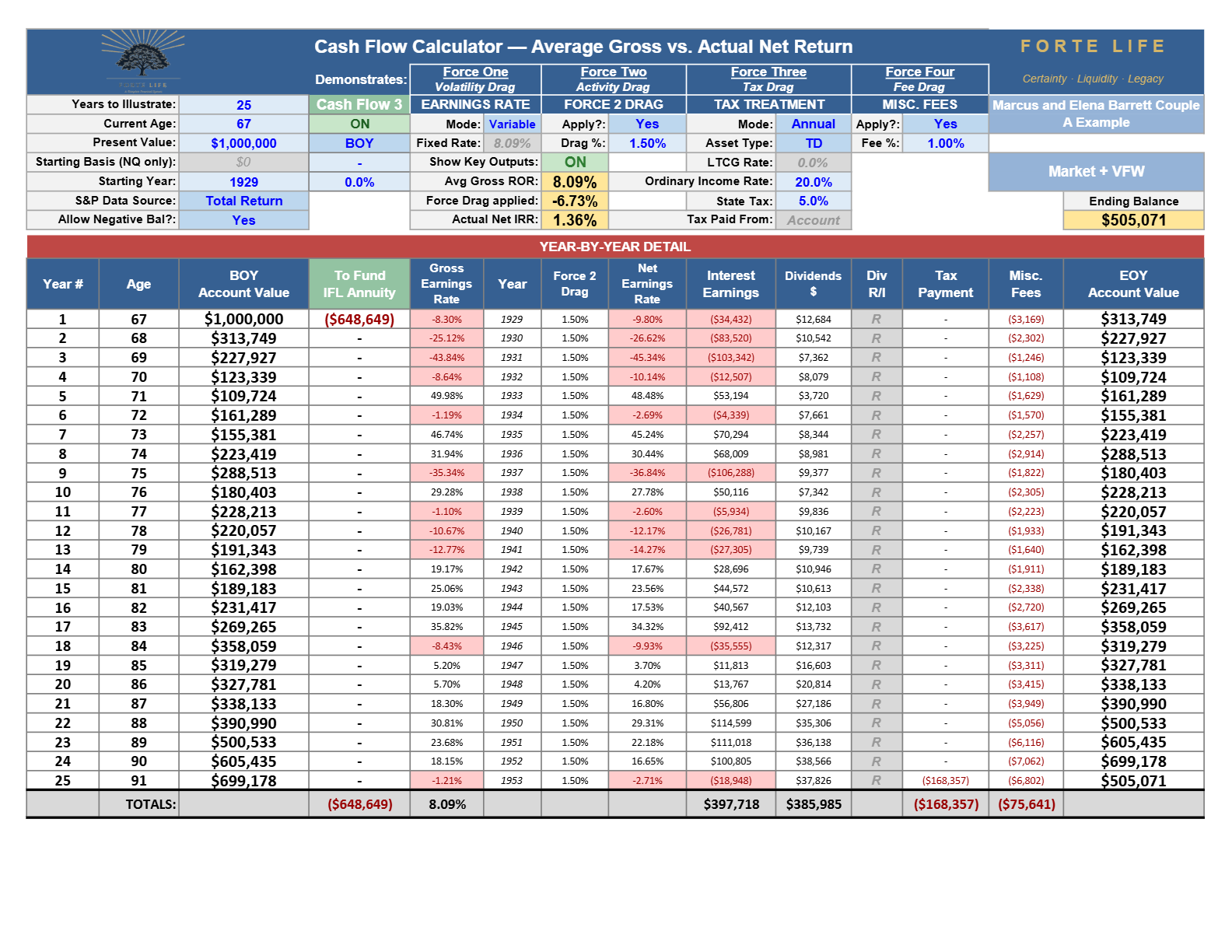
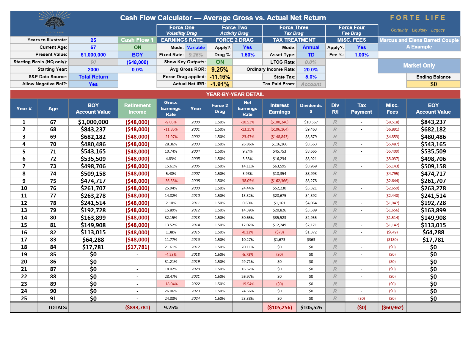
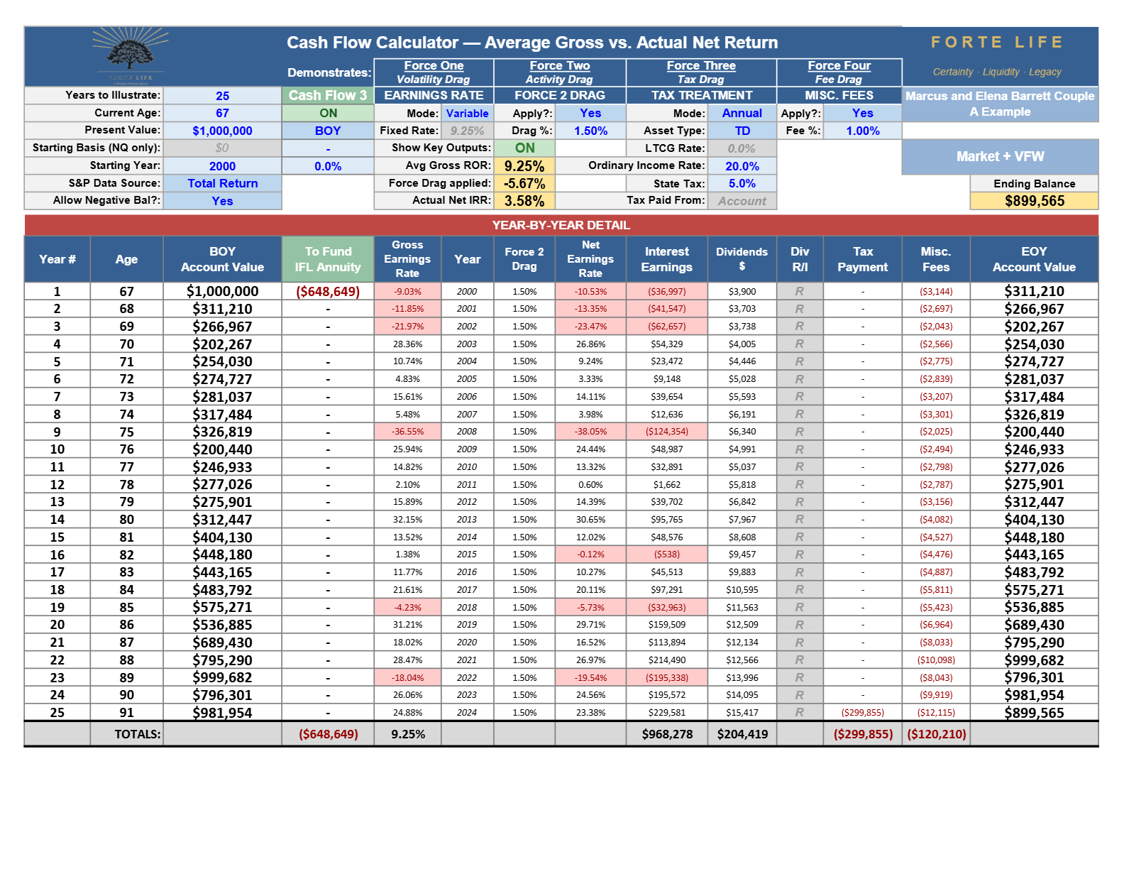
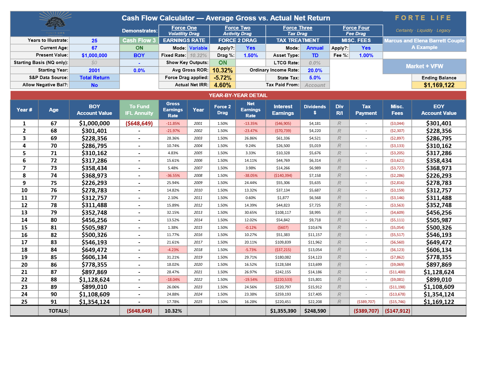
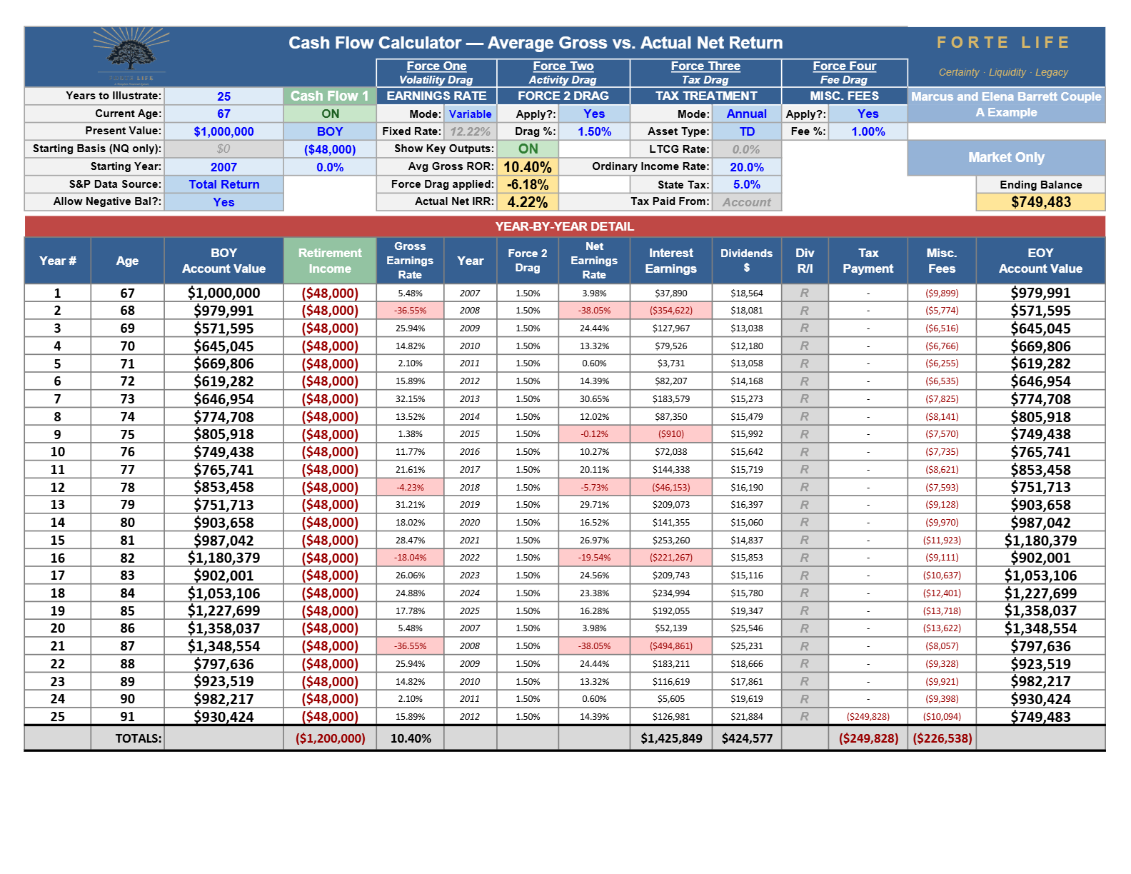
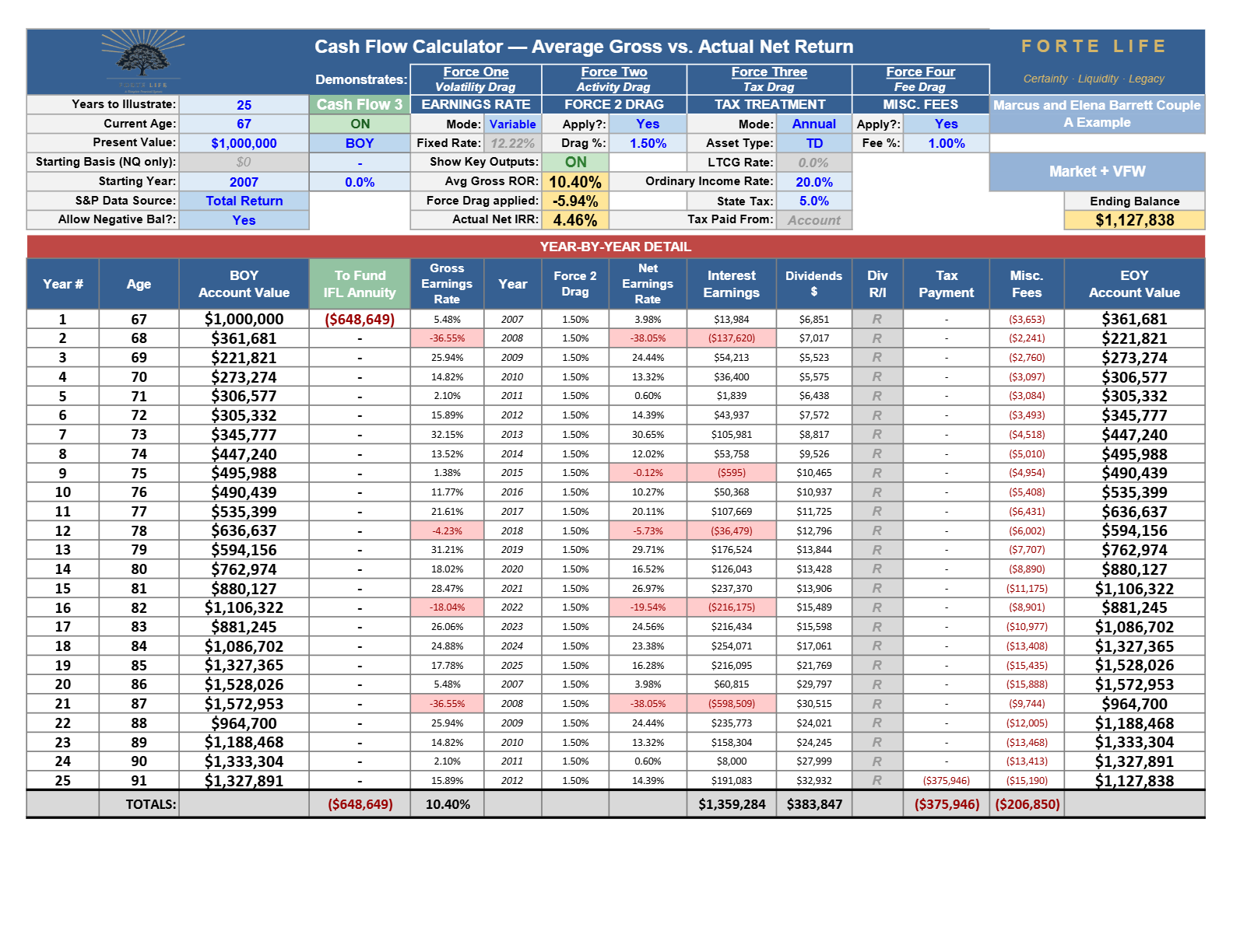
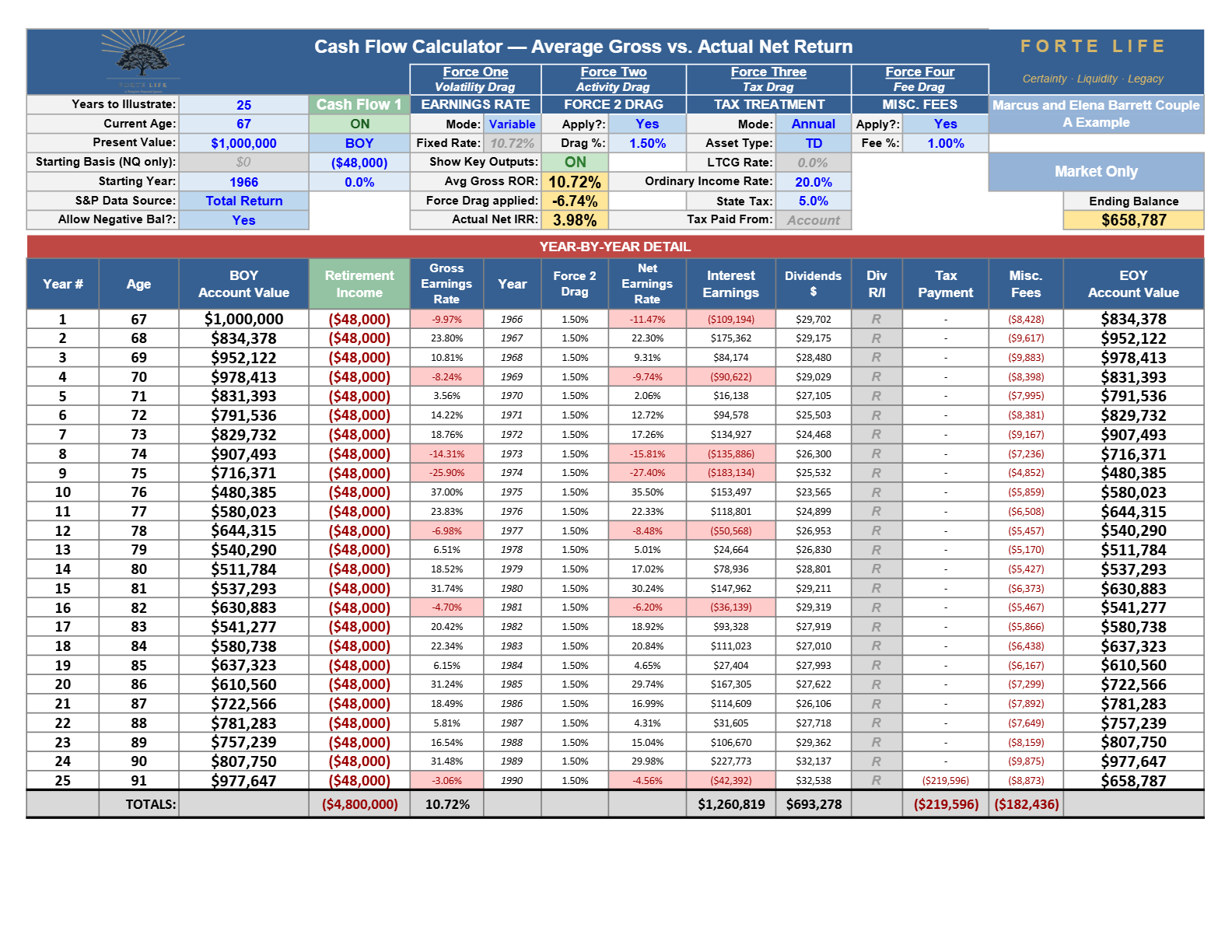
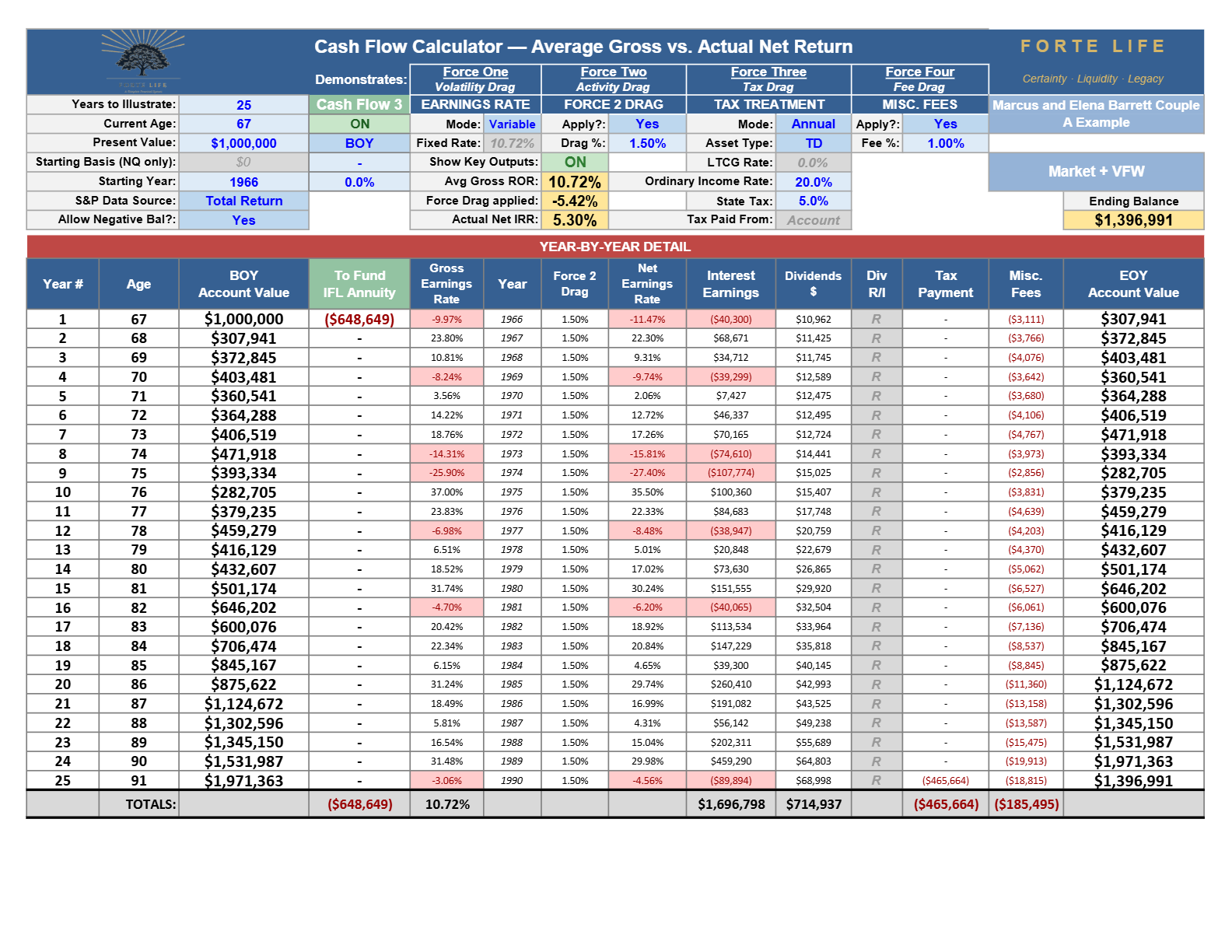
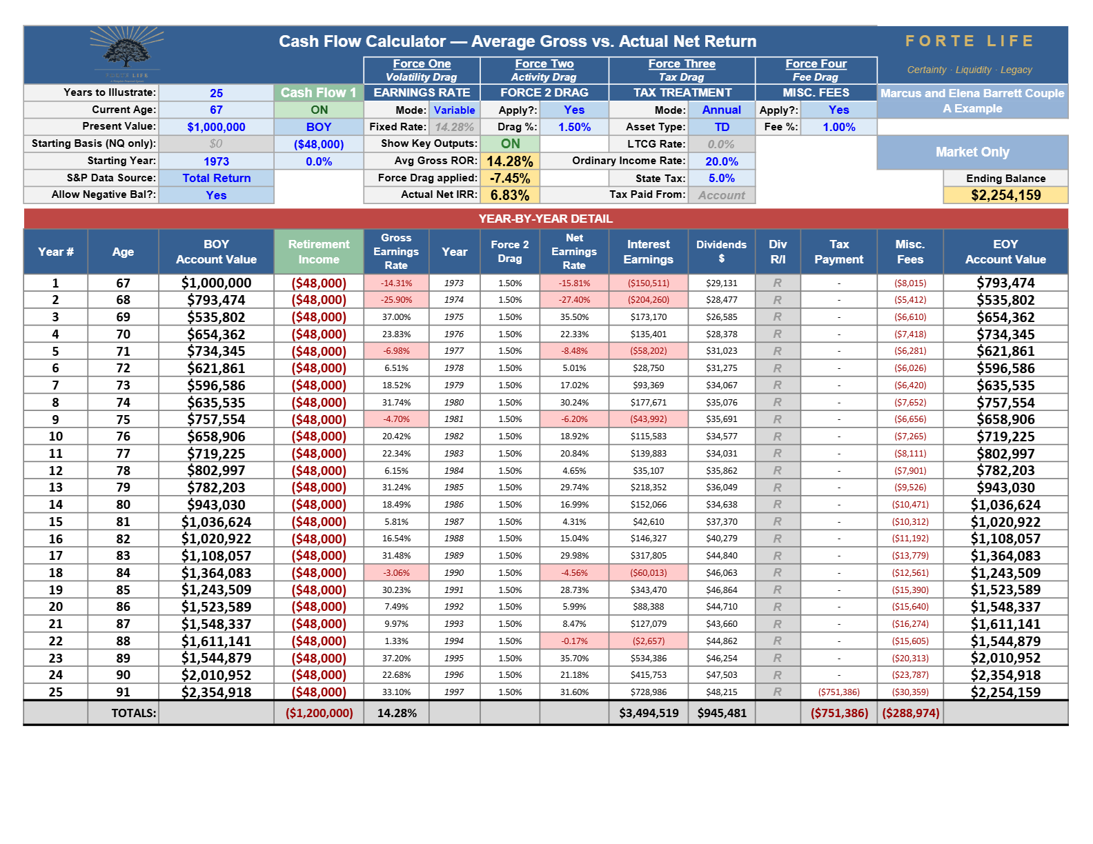
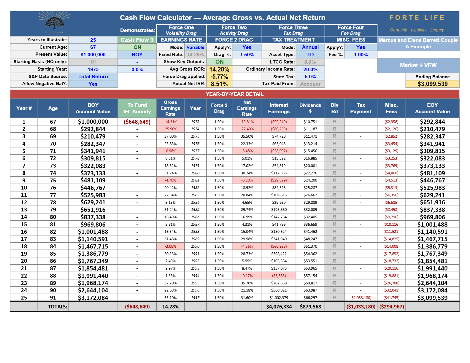
The actual Forte Life Cash Flow Calculator export, year by year, with all four forces applied — never retyped.
1929 — the Depression.
Market-only — income stops at age 78 after $540,146; the 1929–1932 collapse empties the account in twelve years.
Market + Firewall — full $48,000 for life, remainder ends $505,071. (the $648,649 premium leaves in year 1 to fund the joint lifetime annuity; the remainder is then never drawn and simply recovers. Per the no-piece-rate rule the remainder's isolated internal rate is withheld — it is scored by ending value).
2000 — the dot-com collapse.
Market-only — income stops at age 84 after $833,781.
Market + Firewall — full income for life, remainder ends $899,565. (the $648,649 premium leaves in year 1 to fund the joint lifetime annuity; the remainder is then never drawn and simply recovers. Per the no-piece-rate rule the remainder's isolated internal rate is withheld — it is scored by ending value).
2001 — the worked window.
Market-only — income stops at age 90 after $1,133,599 — this is Exhibit 4·A.
(the market-only 2001 run is rendered in full as Exhibit 4·A above; not reprinted)
Market + Firewall — full income for life, remainder ends $1,169,122. (the $648,649 premium leaves in year 1 to fund the joint lifetime annuity; the remainder is then never drawn and simply recovers. Per the no-piece-rate rule the remainder's isolated internal rate is withheld — it is scored by ending value).
2007 — the financial crisis.
Market-only — survives — pays the full $1,200,000 across the window, ends $749,483.
Market + Firewall — full income for life, remainder ends $1,127,838 — ahead by roughly $378,000, income continuing past the window. (the $648,649 premium leaves in year 1 to fund the joint lifetime annuity; the remainder is then never drawn and simply recovers. Per the no-piece-rate rule the remainder's isolated internal rate is withheld — it is scored by ending value).
1966 — the stagflation bear.
Market-only — survives — pays the full $1,200,000, ends $658,787.
Market + Firewall — full income for life, remainder ends $1,396,991 — ahead by roughly $738,000. (the $648,649 premium leaves in year 1 to fund the joint lifetime annuity; the remainder is then never drawn and simply recovers. Per the no-piece-rate rule the remainder's isolated internal rate is withheld — it is scored by ending value).
1973 — the oil shock.
Market-only — survives — pays the full $1,200,000, ends $2,254,159.
Market + Firewall — full income for life, remainder ends $3,099,539 — ahead by roughly $845,000. (the $648,649 premium leaves in year 1 to fund the joint lifetime annuity; the remainder is then never drawn and simply recovers. Per the no-piece-rate rule the remainder's isolated internal rate is withheld — it is scored by ending value).
Two methodology notes travel with this record. First, a start-year that does not leave a full twenty-five-year historical window is run forward through the most recent year, then repeats from its own start to fill the remainder — 2007, for instance, runs forward through 2025 and then repeats from 2007 through 2012: "2007 and beyond, then repeating itself when necessary." Second, the annuity contract's terms — the 7.40% joint lifetime payout — are held constant across every start-year on purpose. Applying today's contract to 1929, 1966, or 1973 is anachronistic, and deliberately so: the point of the record is to vary only the market sequence the remainder faces, holding the instrument fixed, so the difference each row shows is the sequence's doing and nothing else.
Here is what the record produced. The table is my synthesis; the figures are the outputs of the runs above.
| Retiree start-year | Market-only — income paid, then ending | Market + Firewall — income paid, then ending |
|---|---|---|
| 1929 — Depression | $540,146, stopped at 78 → $0 | $1,200,000 → $505,071 |
| 2000 — dot-com | $833,781, stopped at 84 → $0 | $1,200,000 → $899,565 |
| 2001 | $1,133,599, stopped at 90 → $0 | $1,200,000 → $1,169,122 |
| 2007 — financial crisis | $1,200,000, survived → $749,483 | $1,200,000 → $1,127,838 |
| 1966 — stagflation bear | $1,200,000, survived → $658,787 | $1,200,000 → $1,396,991 |
| 1973 — oil shock | $1,200,000, survived → $2,254,159 | $1,200,000 → $3,099,539 |
Synthesis table. "Income paid" is what each plan actually delivered across the twenty-five-year window; a market-only account stops paying the year it hits zero, while the Firewall pays $48,000 for life and its income continues past the window. "Ending" is the legacy — for the Firewall, the invested remainder. Every account is floored at zero; no balance goes negative.
Read the table in two parts. The first is the one this section was built for. In three of the six start-years the market-only plan failed — and the honest, realistic way to see a failure is not a negative balance, because an account cannot go below zero. It is the moment the income stopped while the couple was still alive. Starting in 1929, the checks stopped at age 78, after only $540,146 had been paid. Starting in 2000, at 84. In the 2001 window this paper works in, at 90. From the identical $1,000,000, the Firewall plan paid the full $1,200,000 across the window — and keeps paying for life — and still left a legacy. The 2001 case is not the cruel outlier; it sits in the middle of the record, and it is the kindest of the three failures.
The second part is the one these runs uncovered, and it is stronger than "you might run dry." Look at 2007, 1966, and 1973 — the three start-years where the market-only plan survived, paying the full income and ending at $749,483, $658,787, and $2,254,159. Even there the Firewall plan won — leaving $1,127,838, $1,396,991, and $3,099,539, roughly $378,000, $738,000, and $845,000 more — and its income does not stop at the edge of the window the way a drawn-down account eventually must. So the record answers two dismissals at once. "You rigged the window" — no; worse windows exist, and the Firewall plan wins across all of them. And the subtler "but the market usually recovers" — sometimes it does, and even then the household carried a depletion risk it did not need to and left six figures on the table. The Firewall plan is not the plan that wins only when the market fails. It is the plan that wins whether the market fails or not.
5.2 The analysis the industry does not run
There is one comparison left, and it explains why a reader may have heard the exact opposite of everything above — why so much of the financial-services industry markets a market-only approach as superior to a coordinated one. The answer is not dishonesty. It is a modeling choice, and it is visible in a single pair of runs.
Take the 2001 household and run it two ways, changing only one thing — whether the market is modeled as a fixed smooth average (the same 10.32% every year, the other three forces still applied) or as the variable real sequence (the actual 2001–2025 order):
CF Calc: fixed vs. variable, market-only and Firewall. $1,000,000 · −$48,000/yr · four forces · 2001, run four ways — market-only and Firewall, each at a fixed 10.32% and on the variable real sequence. The four runs, rendered. The only variable that changes between the top pair and the bottom pair is fixed-versus-variable; every other input is identical.
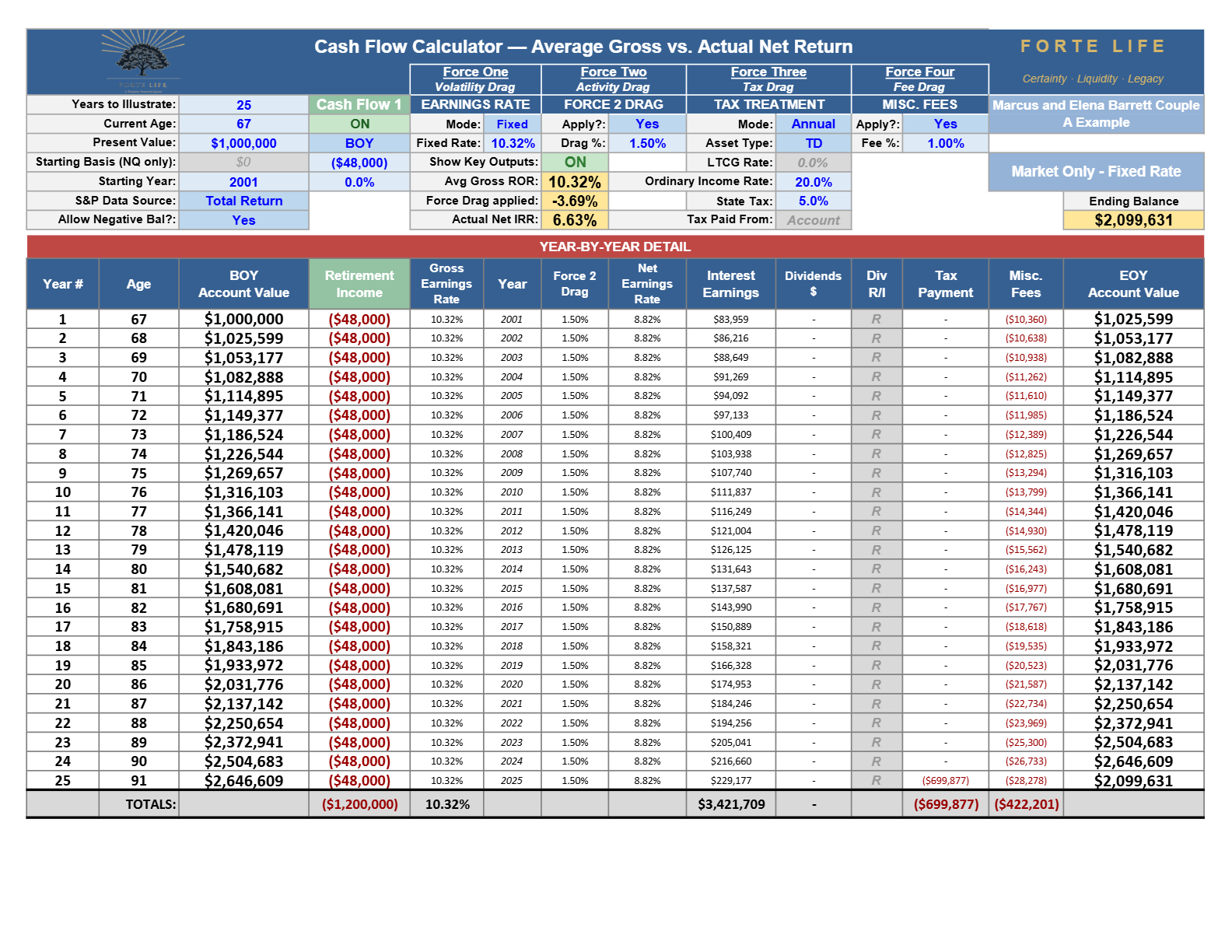
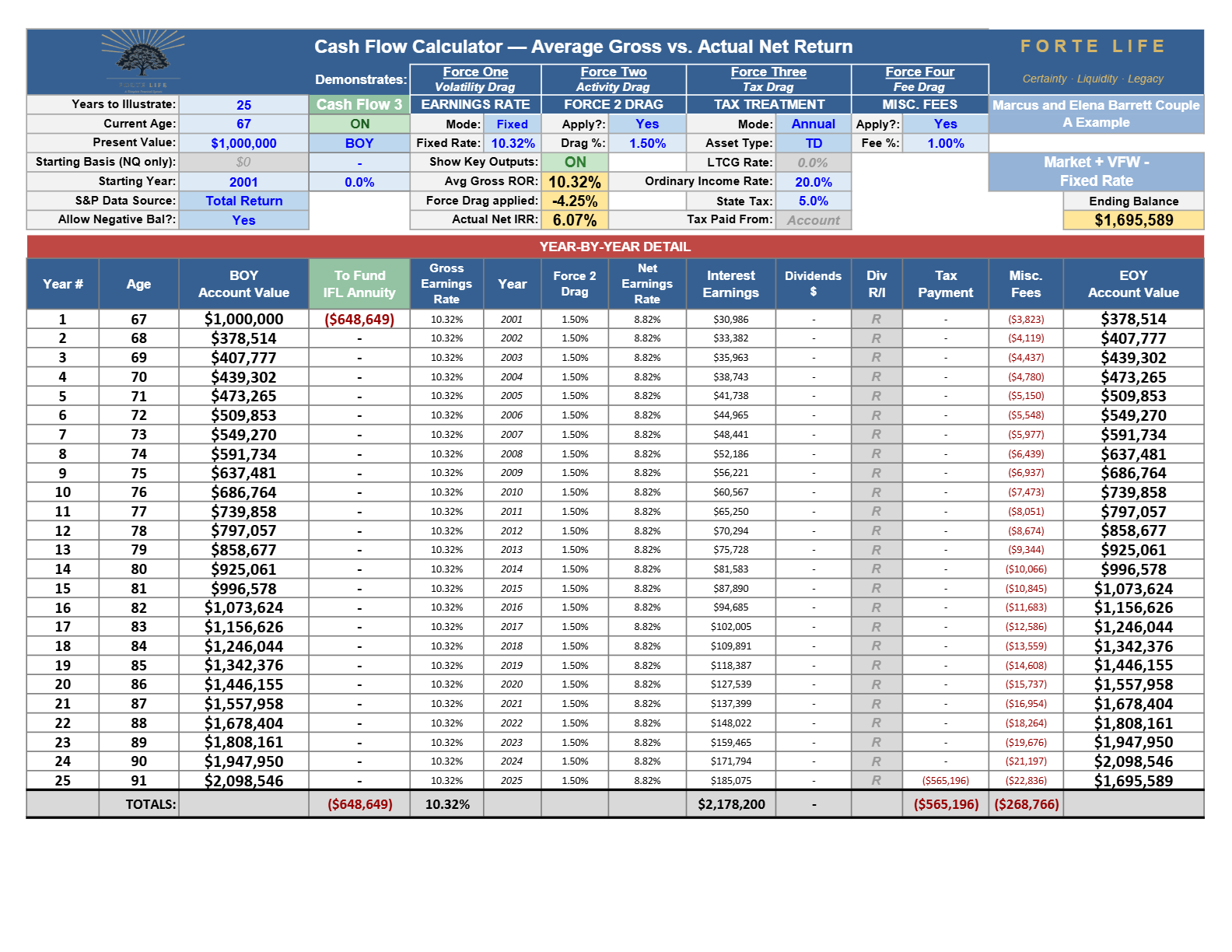
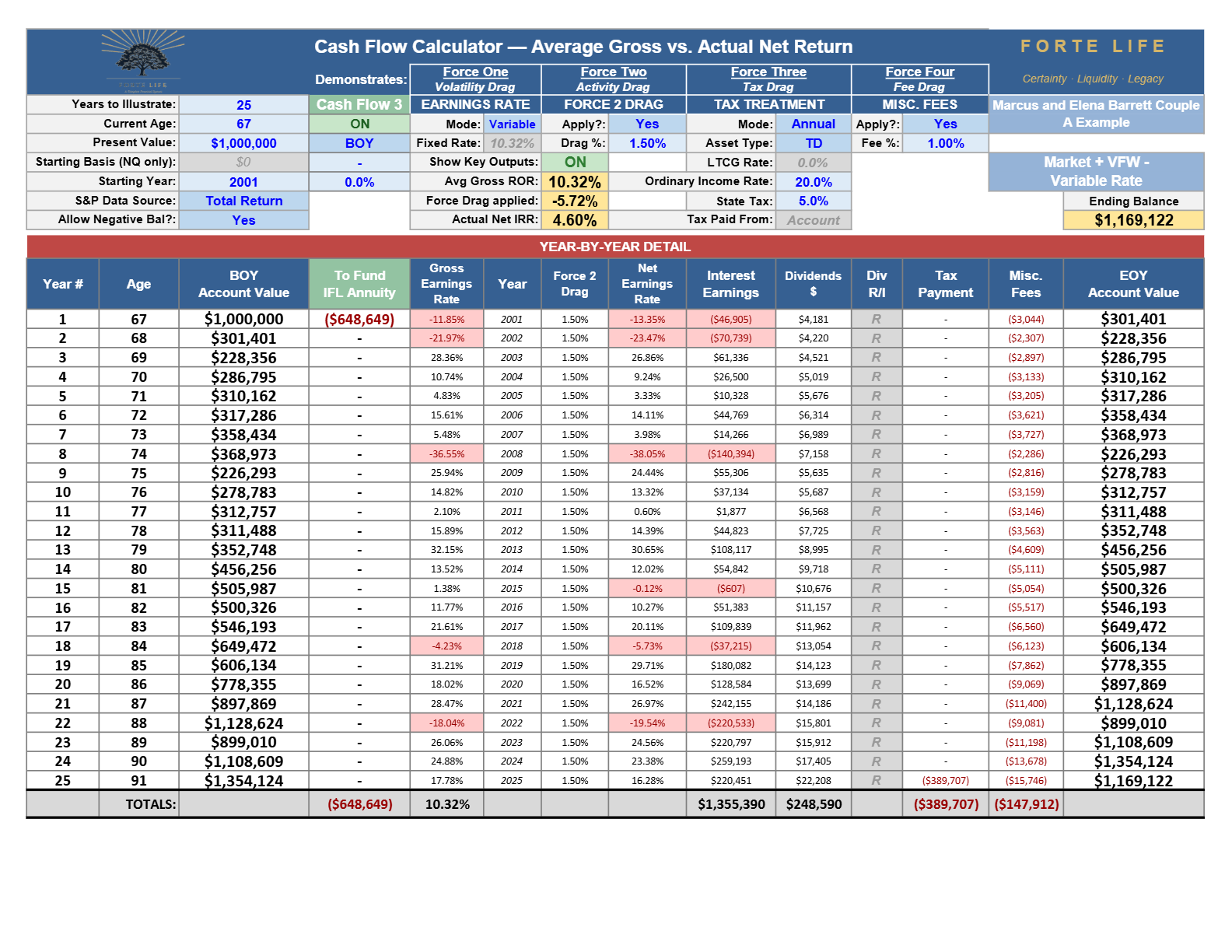
The actual Forte Life Cash Flow Calculator export, year by year, with all four forces applied — never retyped.
Market-only, fixed 10.32% (the smooth projection the industry runs) — ends $2,099,631, never depletes:
Market + Firewall, fixed 10.32% — remainder ends $1,695,589 (piece-rate IRR withheld; scored by ending value):
Market-only, variable real sequence — floored at zero, income stops at 90 after $1,133,599, ends $0 (this is Exhibit 4·A):
(rendered as Exhibit 4·A above; not reprinted)
Market + Firewall, variable real sequence — remainder ends $1,169,122:
| The 2001 household | Market-only — income paid / ending | Market + Firewall — income paid / ending |
|---|---|---|
| Modeled at a fixed 10.32% (smooth average) | $1,200,000 / $2,099,631 | $1,200,000 / $1,695,589 |
| Modeled on the variable real sequence | $1,133,599 / $0 | $1,200,000 / $1,169,122 |
Synthesis table; income-paid and ending are the outputs of the four Exhibit 5·B runs, each account floored at zero.
Read down the two columns and the trap is exposed. On the fixed smooth-average projection, the market-only plan ends about $404,000 ahead of the Firewall plan — and the Firewall looks like a bad trade, a lump of capital surrendered for guaranteed income the smooth model says you never needed. That projection is the one the industry runs. It is not a lie; it is a model — of a market that has never existed, because no market has ever delivered the identical return every year. Change nothing but fixed-to-variable — feed in the real order of that identical average — and the result does not merely narrow. It inverts. The market-only plan that was winning by $404,000 now fails — its income stops at ninety, after $1,133,599, and it ends at $0 — while the Firewall plan it was beating is the one still standing: the full income paid, still paying for life, and $1,169,122 left.
That inversion is the whole thesis of this paper, proved on one household with one variable changed. Sequence-of-returns risk is not a footnote to the market-only case; it is the difference between that case winning and losing. And the reason it stays invisible — the reason "market-only is superior" can be said in good faith — is that the standard retirement projection is built on the fixed line, which is exactly the model in which sequence risk cannot appear. Run the analysis the industry does not run, and the conclusion turns over. It was not the window, and it was not the model — and, as the next section shows, it is not the draw rate either.
5.3 The whole record — every start-year, not six
A careful reader will have counted. This section has leaned on six start-years, and six is a small number against the objection it invites: you chose the six that flatter the coordinated plan. The honest answer is to stop choosing. The last century offers seventy-six rolling twenty-five-year retirements — every start-year from 1926 through 2001 — and the same household can be run through all of them, market-only against coordinated, with nothing selected and nothing omitted. Run that way, the six become the whole record, and the finding does not soften; it hardens.
Two results survive the full distribution, and they are the two that matter.
The first is the guarantee, and it is not a probability at all. Across all seventy-six windows, the market-only plan ran its income dry while the household was still alive in seven of them — one retirement in eleven ended with the checks stopping, at whatever age the sequence happened to empty the account. The Firewall did so in none. Not in a favorable seventy of seventy-six — in all seventy-six, because a contractual lifetime income cannot be reached by any order of returns. The market-only floor fails 9% of the time, scattered across the record with no way to know in advance which retirement draws the short straw; the guaranteed floor fails zero percent of the time, by construction. That is the difference between a plan that usually works and a plan that cannot fail at its foundation.
The second is what the Buffer does to the market money, and here the record is nearly unanimous. Recall the mechanic: in the year after a loss, the discretionary income is drawn from the non-correlated policy reserve instead of the portfolio, so the shares are never sold into the recovery. Run with and without that single rule across all seventy-six windows, and the Buffer improves the market sleeve's outcome in every one of them — because not selling at the bottom is not a bet that sometimes pays, it is an edge that compounds in every history the market has ever produced. On its own the Buffer would have cut the seven income failures to one; with the Firewall carrying the baseline beneath it, the failures go to zero, and the Buffer's whole effect is spent on making the market money last longer and end higher. On the 2001 window that anchors this paper, the same sleeve that emptied at ninety instead survives the window with a legacy intact.
Set beside this, the industry's usual defense of the market-only approach is a Monte Carlo simulation — a machine that runs thousands of invented futures and reports the percentage in which the money survives. It is an honest tool, and it returns the same uncomfortable answer every time for a market-only income plan: a probability of success meaningfully below one hundred percent, which is simply the seven-in-seventy-six restated as a decimal. The industry's response to that shortfall is to prescribe a lower withdrawal rate — to tell the retiree to spend less, so the simulated failures recede. That is the market-only family's only guardrail: self-insurance through under-spending. They give up income to buy a probability. The coordinated plan does not trade income for a probability; it removes the failure from the floor by contract, and hands the household more income while doing it. This paper does not need a thousand invented futures. It has the one record that actually happened, run in full, and the record says what the simulation says — without asking anyone to pretend the future is a spreadsheet of random draws.
It helps to step back from the ledgers here, because there is a plainer way to see the whole choice. Picture retirement as a journey across the country. If speed were the only thing that mattered — how fast you could travel on an open, dry road — nothing beats a racing motorcycle; it is the quickest way to cover ground, full stop. And yet no one plans a cross-country trip on one. Not because it can't win a clear, straight sprint — it can — but because three thousand miles is not a sprint. The route runs through weather no one can see coming; it has to carry the people and the things you are bringing with you; and above all it has to arrive. So people choose the car — a little slower at the top end, and in exchange a windshield, a roof, seatbelts, and room for the family, built to finish the trip in whatever weather is waiting.
And here is what tips the choice from sensible to obvious: you can check the forecast. Not the exact hour each storm will break — no one is given that — but the range of what is coming and the near-term outlook, which is all a traveler ever really has. Read the gauges a retiree can read today and they point one way, toward weather rather than calm. The national balance sheet leaves tax rates far more room to rise than to fall (Section 7). Inflation has shown it is not a settled thing (Section 12). Interest rates move in lurches, and conflict abroad keeps markets on edge. And beneath all of it runs the most forecastable force there is — demographics: the largest generation in American history spent forty years buying equities through the retirement-plan machinery built for exactly that, and has now crossed into the years when income needs and required withdrawals make it a seller, for decades, with no cohort its size behind it to buy. (That reversal — who is buying when your whole cohort is selling — is the subject of the companion "Who's Buying?" analysis; it is named here only to establish that the rough weather ahead is not a guess.) The forecast, in other words, is legible, and it is not benign. What it still cannot tell you is the timing — whether the worst of it lands in your first years of retirement or your last — and timing is the entire game, because a storm in the first years is what empties the account. But read that correctly, because it is not an argument for predicting the weather — it is the reverse. Precisely because the range of what lies ahead is wide and its timing unknowable, the intelligent move is not to wager on a forecast; it is to install the pieces that shrink that range of outcomes and raise the probability of arriving, whatever actually comes. The car does not predict the storm; it makes the trip survivable in all of them — which is the one thing the motorcycle cannot do, and the reason no one takes it across a continent.
A market-only retirement is the motorcycle. On the open, dry stretches — the kind sequences — it is faster, and it will sometimes finish richer than the coordinated plan; this paper will not pretend otherwise. But that is the answer to the wrong question. It measures top speed on a clear road, when the thing that actually decides a retirement is whether you arrive — through the weather that actually comes, whose timing no one can call, with an income that never stops and enough left for the people riding with you. And notice the motorcyclist's only real protection: to slow down — to give up the very speed that was the reason to choose the bike at all. That is precisely the market-only family's guardrail, the lower withdrawal rate a simulation prescribes: ride slower, and hope. The coordinated plan is the car. It trades a sliver of a top end no one can count on for a floor that held in every weather the last hundred years produced. No one rides a motorcycle across the country because it is faster; and no one should cross thirty years of retirement on growth alone because, in the sunshine, it sometimes ends richer.
So the choice the record actually poses is not more legacy or less. It is a paycheck that can stop, or a paycheck that cannot — and, on the market money, a sleeve left to be sold at the bottom, or a sleeve shielded from it. And that is what the seventy-six windows actually measure: not a forecast of the future, but the full range of what has already happened — and how much narrower, higher, and more certain that range becomes the moment the two pieces are in place. Run every start-year the last hundred years contain, and the coordinated plan wins the only two contests that decide whether a retirement holds: the income never fails, and the market money is treated better in nearly every history the record holds.
Every figure in this section traces to the Cash Flow Calculator; the 2001 window is validated to the dollar against Exhibit 4·A, and the full seventy-six-window run is available on request.
It Was Not the Draw RateWhy "You Didn't Run Out" Is Not "You Were Safe"
The last refuge of the market-only plan is the withdrawal rate. Four-point-eight percent was too high; a careful retiree simply draws less, and none of this happens to them. It is true that a lower draw survives longer. It is not true that a lower draw makes a household safe, and the difference between those two things is a lesson worth the whole section.
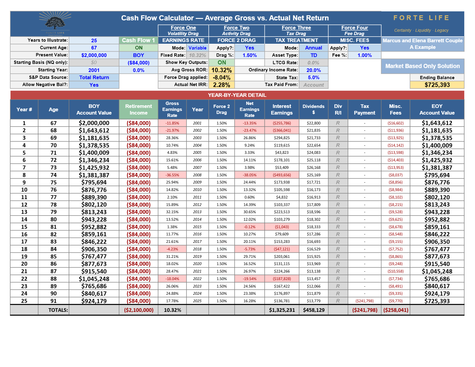
To see it, hold the market constant and vary only the draw — one family, not two. A household retires with $2,000,000 and draws $84,000 a year: a 4.2% withdrawal, more conservative than Section 4's, the kind of number that gets a household told it is in fine shape. Run against the identical 2001–2025 sequence, that account does not run dry.
CF Calc: $2,000,000 at a 4.2% draw (Conventional, market-only). Present value $2,000,000 · age 67 · −$84,000/yr · S&P 500 2001–2025 · four forces as in 4·A. The exported run, rendered below — the account survives the window but never stops being drawn on a shrinking base:
The actual Forte Life Cash Flow Calculator export, year by year, with all four forces applied — never retyped.
Authoritative CF-calc export ($2,000,000 · −$84,000/yr · 2001–2025). Summary outputs: Average Gross ROR 10.32% · Actual Net IRR 2.28% · ending balance $725,393 — the account survives the window; it does not deplete.
But look at how that "success" was lived, because the ending balance hides it. This household began drawing 4.2% of two million dollars and ended drawing roughly 10% of an account that had fallen under $850,000 — the same fixed $84,000 becoming a larger and larger bite of a shrinking base, exactly the Section 3 mechanism, only slower. Along the way it spent down about 64% of its principal and white-knuckled 2008 and 2022 with every income dollar leaving a falling account. It did not run out. It also did not spend a single year of that retirement free of the question. Security curdled into precarity at the very age the household was least able to do anything about it.
Now nudge the need by six-tenths of one percent. Raise the draw to $96,000 — a 4.8% withdrawal on the same $2,000,000, a slightly fuller life or a slightly smaller nest egg — and the identical market takes this household to zero by ninety. That is not a coincidence, and it is the sharpest single point in the paper: $2,000,000 drawing $96,000 is exactly twice $1,000,000 drawing $48,000. Same shape, same 1.04% Actual Net, same dry-at-ninety. The million-dollar account of Section 4 and the two-million-dollar account here are not two different stories. They are the same story at two scales, and the variable that decided both was never the size of the nest egg. It was the draw rate against the order the market delivered.
That is the lesson, and it is this paper in a single line:
"You didn't run out" is not the same as "you were safe."
Sequence risk does not announce itself by emptying an account. It works by making survival hostage to a withdrawal rate the household believed was conservative — so that the whole distance between ending with $725,393 and ending with nothing is six-tenths of one percent, decided by an order no one chose. A plan that "makes it" on a 4.2% draw through a merely-adequate sequence has not solved the problem. It got lucky inside it. Everything from here is about not needing the luck — and it starts with the part of the problem the market-only plan never even names: the tax machine waiting in the distribution phase.
The Distribution-Phase Tax Machine
Sequence risk is the danger every retiree has at least heard named. The tax machine is the one almost none have, and it is the largest untapped differentiator in retirement income planning — because it does not exist during accumulation at all. A saver's tax life is simple: contribute, defer, ignore. A retiree's is the opposite. The day income begins, the tax code stops being a flat background cost and becomes an active machine with thresholds, cliffs, and feedback loops, in which a single dollar of income can trigger costs several times its own size — and in which assets a retiree was told were "tax-free" quietly set the machine off anyway. The companion Accumulation paper cannot cover this; its reader is not drawing income. It is Distribution's to own, and this section owns it.
7.1 Tax-rate risk — the bet inside every deferred dollar
Before any of the machine's gears turn, there is a prior question most savers are never asked: at what rate will the tax-deferred balance be taxed when it finally comes out? Every 401(k), IRA, and 403(b) rests on one unstated premise — defer the tax now, at today's rate, and pay it later, at a lower one. That is not a fact. It is a bet on a future tax rate the saver does not set and cannot control — and it sits underneath everything else in this section, because whatever the torpedo, the cliffs, and the forced distributions below cost a household, they cost it at the rate in force when the money comes out, which is decades away and out of its hands.
This paper does not predict future rates, and it does not need to — but the probable direction is written plainly in the public record, and it is not down. The federal debt has gone from roughly $19 trillion to nearly $40 trillion in about a decade, a near-doubling; the annual interest on that debt now exceeds the entire defense budget, running over a trillion dollars a year and climbing. Social Security, Medicare, and Medicaid each face documented shortfalls, and the demographic arithmetic — fewer workers supporting more retirees — only tightens the vise. A government with obligations that grow every year has just three ways to close the gap: cut spending, grow its way out, or raise taxes. No one can say which it will choose. But set that pressure beside where rates actually sit, and the asymmetry is stark: the top federal rate today is 37%, and by the standard of the last century that is near the floor — the top rate was 70% as recently as 1980, 91% through most of the 1950s, and 94% during the war. Rates were just cut in 2017 and locked in in 2025; there is far more room above today's rates than below them. To defer a lifetime of savings into that backdrop is to bet against the more probable outcome — much to lose if rates rise, little to gain if they merely hold. The saver who deferred everything has placed that bet whether or not anyone told them they were placing it.
The defense is not a counter-prediction. It is diversification across the three ways money can be taxed — the discipline a serious investor already applies to holdings, applied instead to tax treatment:
Tax-deferred — the 401(k), IRA, 403(b): pay later, at whatever rate is in force when you withdraw. The bucket that is the bet.
Taxable — the ordinary brokerage account: pay as you go, at capital-gains rates. Visible and flexible, but inefficient as the dominant vehicle.
Tax-free — Roth accounts and properly structured permanent life insurance: pay the tax up front, and every later withdrawal, structured correctly, arrives with no further federal income tax no matter where rates have moved.
The advantage is not merely owning all three buckets; it is holding the right balance across them — and that balance is built deliberately, with a runway. Which dollars are converted and which are left to defer, how much tax-free capacity is funded and by when — these are decisions that reward being made in advance. A household that positions its buckets in the years before the paychecks stop arrives at retirement with an income plan already coordinated for tax efficiency, rather than reacting to the machine one forced withdrawal at a time; the greatest leverage belongs to the reader with years still to position. But it is never too late to make a difference. Many readers are at the door of retirement, or already through it, and for them the levers are not gone — they are simply nearer at hand. Repositioning that begins at sixty-seven, or seventy, still lowers the tax on the years ahead, still shrinks the forced-distribution problem before it compounds, and still moves income into the bucket the machine cannot reach. The right question is never "am I too late," but "what does my plan hold in each bucket today, what is it likely to cost at the rate that is coming, and what can still be moved" — because planning for tax efficiency pays now and for every year that follows. A coordinated plan does not merely hold the tax-free bucket; it fills it deliberately, on a schedule the household controls, which is the lever 7.7 returns to. That is tax-rate risk, and it is the ground the rest of this section stands on.
7.2 Provisional income — the hidden meter behind Social Security
Most retirees believe Social Security is tax-free, or nearly so. For a household with any meaningful other income, it is not — and the mechanism is one almost no one has seen. The IRS does not look at your Social Security benefit directly; it looks at a figure called provisional income, which is your adjusted gross income plus any tax-exempt interest plus one-half of your Social Security benefits. Where that figure lands decides how much of your Social Security itself becomes taxable:
For a married couple filing jointly, below $32,000 of provisional income, none of the benefit is taxed.
Between $32,000 and $44,000, up to 50% of the benefit becomes taxable.
Above $44,000, up to 85% of the benefit becomes taxable.
Here is the detail that turns this from a footnote into a machine: those thresholds have never been adjusted for inflation. They were written in the 1980s and 1990s and fixed in place. A $44,000 line drawn four decades ago catches almost every retiree with a funded 401(k) today, and it catches more of them every year, because the line does not move while incomes do. This is not a high-income problem. It is a middle-income certainty.
7.3 The Social Security tax torpedo
The reason provisional income matters so much is not the tax on the Social Security benefit by itself. It is what that tax does to the marginal cost of every other dollar of income while a household is inside the phase-in range. Because each additional dollar of ordinary income can pull an extra fifty or eighty-five cents of Social Security into taxation alongside it, the true marginal rate on that dollar is not the bracket the retiree thinks they are in — it is that bracket multiplied.
The effect has a name among the advisors who know it: the tax torpedo. Its size depends on where in the provisional-income range the household sits. In the lower band — where each extra dollar of income makes an additional fifty cents of Social Security taxable — a retiree who believes they are in the 12% bracket already faces a real marginal rate of 18% (12% × 1.5). Deeper in the range, where each dollar pulls eighty-five cents of benefit into taxation, that same 12% bracket faces 22.2% (12% × 1.85) — nearly twice its face value. A household in the 22% bracket can face a real marginal rate near 40.7% by the identical mechanism (22% × 1.85). The retiree drawing "a little more from the IRA this year" to cover a roof or a car has no way of seeing, on any statement, that the dollar cost them forty cents rather than twenty-two. The meter is running, and it is not printed anywhere.
Watch it work on one household. Take a married couple, both sixty-nine, retired, filing jointly, who between them collect $48,000 a year in Social Security and draw $30,000 from a traditional IRA to top up their spending. Their provisional income is the IRA draw plus half the Social Security — $30,000 + $24,000 = $54,000 — already past the $44,000 line, so they sit in the 85% band. Now the roof needs replacing, and they pull an extra $10,000 from the IRA to pay for it. That $10,000 is ordinary income — but it does not travel alone. Because every additional dollar in this range drags 85 cents of Social Security into taxation with it, the $10,000 draw makes an additional $8,500 of their Social Security taxable. Their taxable income rises not by $10,000 but by $18,500, and at the 12% bracket they believe themselves to be in, the tax on that is $2,220. The $10,000 roof cost them $2,220, not $1,200 — a real rate of 22.2%, the 1.85× above made concrete — and nothing on any statement told them the difference. (The multiplier holds while the household is inside the phase-in range and below the 85% cap.)
7.4 The IRMAA cliffs
The second gear of the machine is Medicare. Higher-income beneficiaries pay a surcharge on their Medicare Part B and Part D premiums, the Income-Related Monthly Adjustment Amount — IRMAA. Three features make it dangerous in ways an income-tax bracket is not:
It is a cliff, not a ramp. Cross a threshold by a single dollar and the entire surcharge for that tier applies at once. There is no phasing in. One dollar of extra income can cost a household well over a thousand dollars a year, and at the higher tiers several thousand — for that one dollar.
Both spouses pay, and it stacks on Part B and Part D. The surcharge is per beneficiary, so a married couple pays it twice, on two kinds of premium.
It looks back two years. Your IRMAA today is set by your income from two years ago, so a one-time income event — a large IRA withdrawal, a Roth conversion done carelessly, the sale of a property, a sequence-forced liquidation in a bad market year — raises your Medicare premiums for a year you have already lived and can undo only through a discretionary appeal.
The exact thresholds and surcharge amounts are published annually and shift with inflation, so a live plan uses the current figures; the mechanism is what matters here, and the mechanism is a staircase of cliffs sitting directly in the path of any retiree whose income is lumpy or whose required withdrawals are large.
To see the cliff in dollars, take a couple sitting exactly at the first threshold — at the figures in force for 2025, a modified adjusted gross income of $206,000 for a married couple filing jointly. There they each pay the standard Part B premium and no surcharge at all. Let one additional dollar of income arrive — a slightly larger RMD, a capital gain, a Roth conversion misjudged by a hair — carrying them to $206,001, and both spouses cross into the first surcharge tier at once. The surcharge is $74.00 a month per person on Part B and $13.70 a month per person on Part D — $87.70 each, two people, twelve months: $2,104.80 a year. One dollar of income, $2,104.80 of new Medicare cost — and, because IRMAA looks back two years, billed in a year already lived and difficult to undo — the government permits an appeal only for specific life-changing events, granted at its own discretion, so a revision after the fact is not something to rely on. (Those dollar amounts are the 2025 figures and re-set annually; the cliff itself is permanent.)
7.5 "Tax-free" is not "MAGI-free" — the distinction almost no one is shown
Both machines above run on the same kind of fuel: a measure of income that is broader than "taxable income." Provisional income adds back tax-exempt interest; IRMAA runs on modified adjusted gross income, which is adjusted gross income plus tax-exempt interest. That single add-back is where a great deal of conventional retirement advice quietly fails.
Consider the retiree who was told to hold municipal bonds because the interest is "tax-free." It is true that municipal interest escapes federal income tax. It is also true that it counts, in full, toward provisional income and toward IRMAA's MAGI — so the "tax-free" muni can still push a household's Social Security into taxation and still knock it over an IRMAA cliff. Tax-free, it turns out, is not the same as invisible to the machine. Very few of the assets marketed to retirees as tax-advantaged are actually MAGI-free.
Two kinds of income are. Qualified distributions from a Roth account do not enter adjusted gross income, so they touch neither provisional income nor IRMAA. And income drawn properly from a properly structured whole life policy — through withdrawals to basis and then policy loans — is likewise not a taxable event and does not enter those figures. The table below sorts the common retirement income sources by what the machine actually sees. It is a reference, not a calculator output.
| Income source | In taxable income? | In provisional income (Social Security)? | In MAGI (IRMAA)? |
|---|---|---|---|
| Traditional 401(k) / IRA withdrawal (incl. RMDs) | Yes | Yes | Yes |
| Qualified (rollover) annuity income | Yes | Yes | Yes |
| Capital gains / taxable dividends | Yes | Yes | Yes |
| Municipal bond interest ("tax-free") | No | Yes | Yes |
| Qualified Roth distributions | No | No | No |
| Properly structured policy income (basis + loans) | No | No | No |
Row discipline: a qualified annuity — one funded by a rollover of pre-tax 401(k) money, which is the Firewall in this paper's central exhibits — produces fully taxable income that does count in these figures. Its advantage in the machine is not invisibility; it is described in 7.7.
7.6 RMDs — the machine on a timer
There is one more gear, and it is on a clock the retiree does not control. Beginning at age seventy-three, required minimum distributions force a rising percentage of every traditional 401(k) and IRA out of the account each year, taxed as ordinary income, whether or not the retiree needs the money and whether or not it is a good year to sell. The penalty for taking too little is severe. For a household that saved diligently into tax-deferred accounts — which is most of them — the RMD is a taxable-income event that arrives every year, grows as a share of the balance with age, and lands directly on provisional income and on IRMAA's MAGI. The tax-deferred account that felt like a gift during accumulation reveals, in distribution, that a silent partner has been waiting inside it the whole time, and that the partner sets the schedule.
How fast the partner's share rises is worth seeing on one balance. Take a $1,000,000 traditional IRA and hold the balance flat, so the only thing moving is the IRS's own divisor — the Uniform Lifetime Table factor that shrinks with age:
| Age | IRS divisor | Forced withdrawal on $1,000,000 | As a % of the balance |
|---|---|---|---|
| 73 | 26.5 | $37,736 | 3.8% |
| 75 | 24.6 | $40,650 | 4.1% |
| 80 | 20.2 | $49,505 | 5.0% |
| 85 | 16.0 | $62,500 | 6.3% |
| 90 | 12.2 | $81,967 | 8.2% |
| 95 | 8.9 | $112,360 | 11.2% |
Illustrative — the balance is held at $1,000,000 to isolate the rising divisor; a real balance moves, but the forced percentage climbs exactly like this regardless. Divisors are the current Uniform Lifetime Table.
Every one of those forced dollars is ordinary income, and every one lands on provisional income and on IRMAA's MAGI. The retiree who needed only $40,000 to live at eighty-five is required to withdraw $62,500 anyway — and to run the whole tax machine on the difference, whether the money was wanted or not.
And the machine does not switch off when the retiree dies — it is handed to the next generation, usually at a worse rate. A household that takes only its required minimum each year, precisely to hold down its own tax bill, leaves behind the largest possible tax-deferred balance — and under current law an adult child who inherits it can no longer stretch the withdrawals across a lifetime. The account must be emptied within ten years. Because the parent had already begun taking RMDs, the heirs must take an annual distribution in each of years one through nine and clear the entire remaining balance by the end of the tenth — every dollar of it ordinary income, arriving in what are usually the children's own peak earning years, and therefore likely taxed at a higher rate than the parents would ever have paid. "Take only the minimum" does not defuse the tax-deferred account; it forwards it to the very people the money was meant for, enlarged and on a ten-year clock. (These are the current post-SECURE-Act rules; a live plan uses the schedule then in force.)
7.7 Why a coordinated plan is built for the machine and a market-only plan is not
Put the gears together and the shape of the problem is clear: a market-only, tax-deferred plan feeds the machine on every axis at once. Its income is all ordinary and all MAGI-counting; its withdrawals are lumpy, because sequence risk forces larger draws in exactly the bad years; its RMDs are non-negotiable and rising; and its "safe" muni holdings do not escape the meters. The retiree is not doing anything wrong. The structure is simply built to trip every threshold the distribution phase contains.
A coordinated plan is built the other way, and it manages the machine on three levers a market-only plan does not have. First, the Firewall converts a slice of the tax-deferred balance into a level, predictable lifetime income — which does not remove that income from MAGI (a qualified annuity's payments are ordinary income), but does eliminate the sequence-driven spikes, so the household stops being thrown over a cliff by a bad market year. It also satisfies the required minimum distribution on the annuitized balance automatically; and because that balance is itself qualified IRA money, its level payments can be coordinated to help satisfy the RMD owed on the household's other IRA assets as well — so a single contract both levels the income and absorbs an RMD obligation that would otherwise force lumpy, machine-tripping draws elsewhere. (A live plan coordinates the specifics with the aggregation rules then in force.) Second, the Buffer — properly structured policy income — is genuinely MAGI-invisible, giving the household a source of discretionary and emergency income it can draw in a high-income year without moving provisional income or IRMAA at all. Third, and most directly against the tax-rate risk of 7.1, the coordinated plan repositions tax-deferred balance into the tax-free bucket on purpose, and on a schedule. Rather than wait for a low-income year — which a household needing $144,000 from the first day of retirement never actually gets — it runs Roth conversions deliberately in the early retirement years, filling the 22% and, where it pays, the 24% bracket on purpose, moving a decade or more of future income out of the tax-deferred account before RMDs, the torpedo, and an unknown future rate schedule can compound on it. Done across the first several years, this can carry a household's later effective rate to 10% or below; taken far enough, to zero — mitigating tax-rate risk and, at the limit, eliminating it. The Firewall's level income is what makes the room to convert without breaking the paycheck. And there is a particularly clean version of the move: because the money funding the Firewall is qualified IRA money, the immediate-income annuity that holds it can itself be structured as a Roth — so that once the up-front conversion tax is paid, the income it pays for life arrives tax-free and invisible to provisional income and MAGI at the same time, the one combination the entire machine cannot touch. None of these is exotic. Each is simply a lever that exists only once a plan has been designed for the distribution phase rather than extended into it on autopilot.
7.8 The same lifestyle, two tax bills — where the machine actually bites
Put the whole machine on two households living the identical retirement, to see what "MAGI-invisible" is worth in dollars. Each couple collects $50,000 of Social Security and wants $50,000 more to spend — $100,000 of lifestyle, the same for both. The only thing that differs is where that extra $50,000 comes from.
| One $100,000 lifestyle, two sources | Market-only household | Coordinated household |
|---|---|---|
| Social Security | $50,000 | $50,000 |
| The other $50,000 is drawn from | a traditional IRA (taxable) | properly structured policy income — basis, then loans (not a taxable event) |
| Provisional income | $50,000 + $25,000 = $75,000 | $0 + $25,000 = $25,000 |
| Social Security pulled into tax | up to 85% — about $42,500 | $0 — none of it |
| Taxable income created | ≈ $92,500 | $0 |
Synthesis table; illustrative, at current statutory thresholds. Policy income drawn as withdrawals to basis and then loans is not a taxable event and does not enter adjusted gross income; the trade is that outstanding loans reduce the eventual death benefit, which the coordinated plan sizes for from the start.
Same house, same trips, the same $100,000 spent. One couple created $92,500 of taxable income and watched $42,500 of its Social Security dragged into tax; the other created none and kept its Social Security whole. Neither household earned a dollar more than the other. The only thing that differed was the address the $50,000 was drawn from — and the tax machine reads addresses, not lifestyles. This is the mechanism the Buffer quietly exploits every time it substitutes policy income for a portfolio draw: it is not only sparing the market sleeve, it is drawing from the one source the machine cannot see.
That is the tax machine, and it is the half of the retirement income problem that has nothing to do with the market at all. The other half — the market — is where the two systems come in, and the first of them is the one that needs no runway.
The Volatility FirewallGuaranteed Income, and Why No One Is Too Late
If the problem is that the market cannot be trusted to deliver income in a reliable order, the first move is not to find a better-behaved market. It is to take the part of the income that must arrive no matter what and remove it from the market's jurisdiction entirely. That is the Volatility Firewall — and because the name has a well-known prior meaning that is nearly the opposite of this one, the distinction travels with it on first use: this income does not manage market risk; it removes your baseline income from the market's jurisdiction entirely. Elsewhere "firewall" has described diversification — spreading a portfolio to contain a loss inside it. This does the reverse. It does not contain a loss; it makes a portion of income unreachable by the market at all. The fire can burn; it cannot cross to the money you live on.
8.1 Why only an insurer can promise it — the mortality-pooling mechanism
The instrument behind the Firewall is a guaranteed lifetime income annuity, and the word guaranteed is earned here for a reason worth building out, because it is the reason no market account can do this job at any rate of return. An individual account holds only its own dollars. To fund income to age one hundred it must be sized for age one hundred — and if the retiree lives to one hundred and three, it fails anyway, because it has no way to know in advance how long it must last. An insurer solves the one problem the individual cannot: it pools mortality across thousands of contract-holders. In any large pool, some will die early and some late, but the average is knowable with actuarial precision even though no single life is. The pool pays every member as though they will live long, and funds the ones who do partly from the ones who do not. That transfer — from the pool of the short-lived to the individual who lives long — is the mortality credit, and it is real money that has no equivalent anywhere in a portfolio.
There is a plainer name for this machine, and it is one most people already trust: a pension. A traditional pension pays for life by pooling mortality in exactly this way, and no one ever accused their pension of being a poor deal for "not getting it all back." A guaranteed lifetime annuity is simply a pension a household builds for itself, in an era when few employers still hand one down.
The mortality credit is why the payout rate on a lifetime annuity exceeds any withdrawal rate a prudent household could safely take from its own account. In the central exhibit below, a joint lifetime contract pays 7.40% of the premium every year for both spouses' lives. No self-funded account can sustain a 7.4% draw across an unknown lifespan — Sections 4 through 6 are the proof of what trying does. The annuity can, not because it earns more, but because it is the only structure that can promise a payment for exactly as long as you live and not one year less. That is the precise sense in which "guaranteed" is an earned word and not a borrowed one, and it is reserved in this paper for exactly that — a contractual lifetime income, and a policy's contractual floor — never for a dividend, an illustrated value, or a market return.
8.2 The Firewall needs no runway — the exhibit, as a scorecard
Here is the claim that matters most to the reader who has quietly decided this paper is not for them because they are already at the door: the Firewall requires no runway. It is not built over years. It is switched on with a single rollover at retirement and produces guaranteed income that same day.
Take the exact household from Section 4 — the $1,000,000 that runs dry at ninety — and change one thing. Instead of drawing $48,000 a year out of the market, roll a portion of the million into a joint lifetime income annuity at sixty-seven. The contract pays the full $48,000 a year for both lives, guaranteed, from day one; the remainder stays invested and, no longer being drawn for income, is free to ride the same brutal 2001–2025 sequence and simply recover.
CF Calc: the market remainder, left to recover. Present value $1,000,000, less $648,649 rolled to the annuity at BOY; remaining balance invested with no income withdrawals; S&P 500 2001–2025; four forces as in 4·A. The exported remainder run, rendered below: the $648,649 premium leaves in year 1 to purchase the annuity, and the remaining balance is then held with no income drawn (the $48,000 comes from the annuity, outside this sleeve), so it rides the identical 2001–2025 sequence and recovers. Per the no-piece-rate rule the remainder's isolated internal rate is withheld; it is scored by its ending value. Terminal after-tax value: $1,169,122 (net of a $389,707 terminal tax).
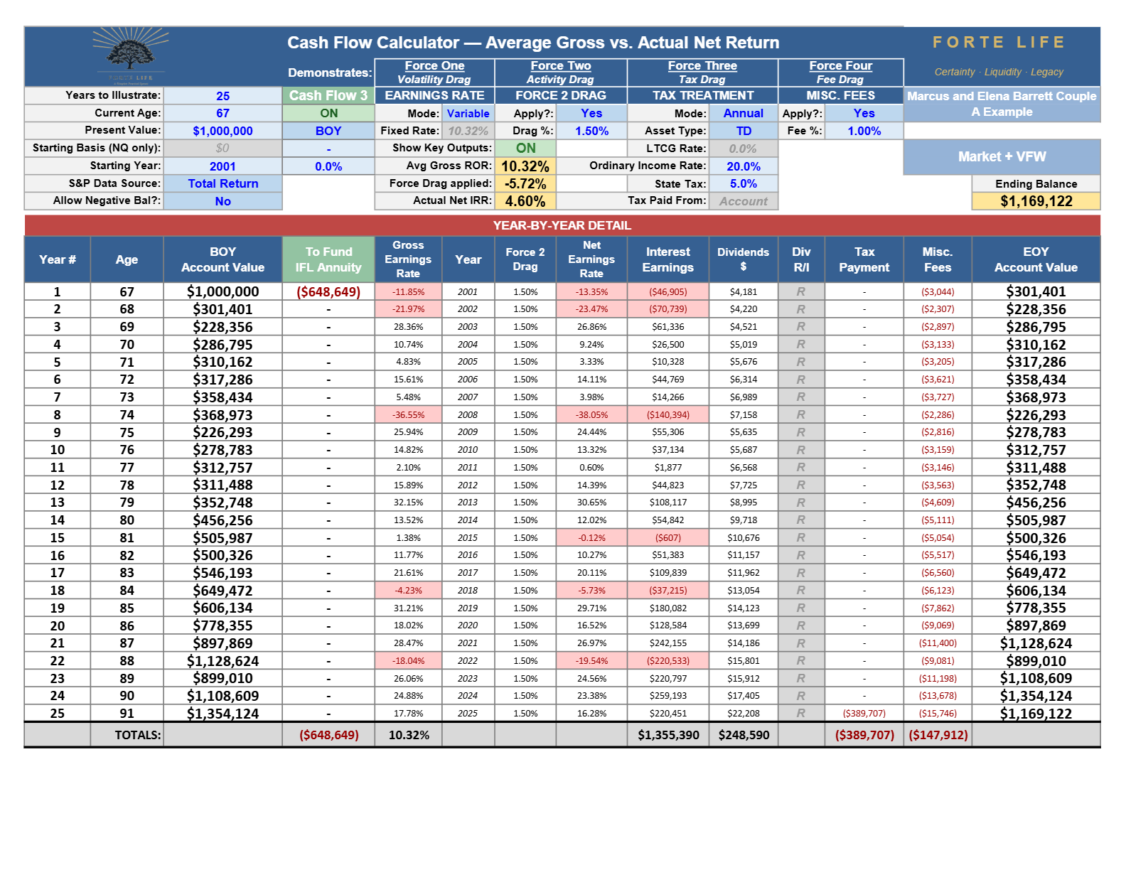
The actual Forte Life Cash Flow Calculator export, year by year, with all four forces applied — never retyped.
Now the discipline this exhibit demands, stated openly because it is the whole thesis of this analysis applied to the one number a reader will reach for. I will not post a rate here. The remainder's standalone return is the internal rate of a piece of a plan, and a piece rate is exactly the rate-contest this body of work refuses — it measures one sleeve in isolation and hides the thing that actually matters. Worse, no single rate could even hold the Firewall's value, because that value is income for life: the annuity's own return climbs the longer the household lives, so any fixed-horizon figure understates it. The honest measure is not a percentage. It is a scorecard — what the same $1,000,000 delivers and leaves:
| The same $1,000,000 at 67 | Conventional (market-only) | Firewall at the door |
|---|---|---|
| Income | $48,000/yr until the account fails | $48,000/yr for life — both spouses, never stops |
| When the income stops | Year 24, at age ninety | Never, while either spouse lives |
| Left to heirs | $0 | $1,169,122 |
| Baseline income exposed to the market | All of it | None |
Synthesis table. Both columns start from the identical $1,000,000; the figures are the outputs of Exhibits 4·A, 8·A, and 8·B.
The same million dollars. One version pays income until ninety and then stops, with nothing for anyone. The other pays $48,000 every year for as long as either spouse is alive and still leaves $1,169,122. Not less income and not less legacy — more of both, from an identical starting balance, with no runway required. The annuity was switched on at sixty-seven.
8.3 The three tiers — "here's your version today, and here's what acting earlier adds"
The coordinated outcome is not one result; it is a ladder of three, and where a household lands depends mostly on how much runway it has — but every rung is far ahead of doing nothing:
| Tier | What it is | Runway required | Result vs. Conventional |
|---|---|---|---|
| 1 — Conventional | Market-only; the account carries all the income and all the risk | — | The baseline: income that can stop, order that decides the outcome |
| 2 — Firewall at the door | Guaranteed lifetime income switched on at retirement; remainder recovers | None | Income for life + a larger legacy than Conventional leaves at all |
| 3 — Full coordinated | Firewall plus a built Volatility Buffer (Sections 9–10) | Years | Everything in tier 2, plus a defended discretionary income and a completed legacy |
Synthesis table.
Read that ladder correctly. The reader at sixty-seven with no runway does not get the Buffer — but they get the Firewall, which is the larger of the two protections and the one that removes the risk to their income outright, and tier two already turns a plan that ends at zero into income for life plus a legacy. The reader with a decade of runway gets both. The framing is never "you missed the top rung." It is: here is your version today, and here is what acting earlier would have added. No one arrives too late to move off tier one — and moving off tier one is the entire distance that matters.
The Volatility Bufferthe Protection That Must Be Built Before It Is Needed
The Firewall removes the risk to the baseline income — the floor a household cannot do without. But most retirements need more than the floor: travel, medical costs, family, the ordinary fullness of a life. That additional income is where a household still wants market growth, and it is exactly the income sequence risk attacks. The Volatility Buffer is the second protection, and it exists for that dollar.
The instrument behind it is the non-correlated cash value of a properly structured whole life policy. That phrase carries weight, so here is what it means in one plain clause: a specific, high-cash-value design — a minimized base policy with a maximized paid-up-additions rider, funded to the edge of the tax line — not the death-benefit-first policy the words "whole life" usually call to mind. It is an asset that earns a contractual return, does not move with the market, and is reachable on demand. How that design works and why its cash value is stable is the subject of the companion Living Asset Strategy paper (The Coordinated Dollar); this paper uses only its buffer property and does not re-derive the instrument. What belongs here is the distribution-phase mechanic — how the reserve is used, how large it must be, and why it cannot be bought once it is needed.
9.1 The mechanic — a year-over-year decision system
The Buffer is not a lump of cash sitting idle; it is a rule the household runs every year, and the rule's precision is what makes it work. The intuitive version — "draw from the safe money in down years" — is subtly wrong and would not survive a careful reader, so state it exactly:
1. A market loss occurs — and that year's income has already been drawn from the portfolio, because no one knows in advance how a year will end. You cannot decide in January to spare a portfolio you do not yet know will fall.
2. The following year, once the loss is a fact, the discretionary income is drawn from the whole life cash value instead.
3. The market portfolio is left untouched, so its recovery works on the full balance rather than one a withdrawal has further reduced.
4. Portfolio withdrawals resume once it has recovered.
The whole effect lives in step two: by drawing the year after a loss from a source that did not fall, the household keeps its shares off the discount rack and lets them ride the recovery. That is the 24.7% problem of Section 3 defused — not by predicting the down year, which cannot be done, but by having somewhere else to draw from once it has happened. This is not a hypothetical: Exhibit 10·B renders the Buffer in action across the real 2001–2025 sequence — five substitution years (2002, 2003, 2009, 2019, 2023), each the year after a market loss, where the income comes from the policy and the market sleeve is left whole to recover.
9.2 How large — the sizing proof, and the question that stays closed
The reserve is smaller than intuition suggests, because it is not sized by how many down years a retirement contains — a typical twenty-five years holds about six — but by the longest unbroken run of them. Across every rolling twenty-five-year window of the last century, the longest unbroken run of down years had a median of two and a maximum of four: the four consecutive years from 1929 through 1932. A three-year buffer covers the longest run in seventy-two of the seventy-six windows; four years covers all seventy-six. So the working figure is three to five years of income held in the non-correlated reserve — sized to cover the longest unbroken run the record holds, and nothing is claimed beyond that coverage.
9.3 Why it cannot be bought once it is needed
A reservoir is dug in the wet years. That is not a detail of how reservoirs work; it is the whole of how they work — water is stored while it is plentiful precisely so there is something to draw when it is scarce, and the one thing you cannot do is dig the reservoir after the drought has arrived. The Volatility Buffer obeys the same law, and it is the fact that makes the Buffer different in kind from the Firewall, and the reason the reader still building should not wait. The second source either exists at the start of the year following a loss, or it does not — and whether it exists was decided years earlier, while the household was still working. A non-correlated reserve of several years' income, built inside a properly structured policy, takes years of funding to reach working strength. A household that begins at fifty-seven arrives at sixty-seven with the structure standing. A household that first hears of it at sixty-seven, in the middle of a downturn, is being handed an umbrella in the rain.
This is the single clearest reason an accumulation-phase decision cannot be graded on an accumulation-phase rate of return. The cash value's job during the working years was never to out-earn the equity sleeve dollar for dollar. Its job was to exist — funded, liquid, and uncorrelated — on the morning a decade later when the market falls in the second year of a retirement. The benefit lives in a different phase than its cost, which is why a single-phase return comparison is structurally blind to it, and why the Buffer is the runway-gated half of the coordinated plan.
Two clarifications keep this from being read as a harder gate than it is, because it is the objection that most often makes a reader think they have already missed their chance. First, the ten-year build in this paper's case study is an illustration, not a minimum. A properly structured policy reaches useful buffer strength in about five to six years of funding, not ten — the full decade in the Barrett case is what makes the exhibit comfortable, not what makes it work. Second, that funding runway does not have to fall before the retirement date; it has to fall before the Buffer is needed — before the first year-after-a-loss that actually calls on it. A household that retires with some other income covering its early discretionary years — a few years of a spouse's continued salary, a bridge annuity, rental income — can be building the Buffer across those same first years and have it standing before the market ever asks for it. A family retiring in three years, with an income source that covers the first three years of retirement, has those three years to build it; the reserve then works across all the years that follow. Nor is the build gated by age the way intuition assumes: a high-cash-value policy can be issued and funded to working strength well into a client's sixties in good health — the oldest case that has worked in practice began at sixty-eight. The rule is not "start ten years early." It is "have it before the year after the loss."
9.4 The success rate — with the Buffer and without
It is fair to ask the question the industry usually answers with a black box: how often does each plan actually work? The honest way to answer it is not a thousand invented futures but the record already run in Section 5 — the same $1,000,000 household, $48,000 a year, started into every notorious retiree beginning the last century offers.
Read as a success rate, the record is stark. The market-only plan delivered its full income across the window in three of the six start-years and failed in the other three — the income stopped while the couple was still alive, in 1929, 2000, and the 2001 window this paper works in. Among the hard starts, in other words, the market-only plan is roughly a coin flip, and the failures are not near-misses: they are years of income that never arrived. The Firewall plan delivered its full baseline income in all six — not because it dodged the bad sequences but because the baseline is guaranteed by contract, so its success rate on the floor is 100% by construction, wholly independent of the order the market delivers. Sequence risk cannot fail a payment the market does not control.
The Buffer does not carry a guarantee, and it should not be described as if it did. What it changes is the contingent part of the plan — the discretionary income still drawn from the market. By moving the draw out of the year after a loss, it keeps the portfolio off the discount rack in exactly the years that decide survival, which is what turns a merely-survivable window into a comfortable one and pushes the marginal windows from failure to survival. In the coordinated case study of Section 10 it fires five times across one window, and the market sleeve ends higher for it every time.
One honest limit travels with this. Six start-years are the worst-case spot checks, not the full distribution; the deepest form of the question runs every one of the last century's seventy-six rolling windows and reports the whole spread of outcomes — which Section 5.3 does in full. But the structural finding does not depend on the count, because it is not statistical — it is contractual: the guaranteed floor succeeds in 100% of futures because no future can reach it, while the market-only floor succeeds only in the futures whose sequence happened to be kind. That is the difference a probability table would only decorate. Which brings the two systems together, in one household, followed across a real retirement.
The Coordinated Planthe Barrett Case Study
The systems of Sections 8 and 9 are, so far, moving parts. This section assembles them into one household, followed across a real retirement, with every figure verified on the calculator and shown as its own exhibit. It is deliberately a more affluent household than the $1,000,000 baseline, because the point here is not the size of the account — it is what a full coordinated plan does when a family has the runway to build all of it. It is tier three.
Meet Marcus and Elena Barrett. They face one fork, not two fates: the same starting point, two roads. The roads are labeled by strategy — the Conventional Plan and the Coordinated Plan — never by anything implying one couple was wiser than the other. Conventional is what almost everyone does, and the reader may well be on it. Read the whole section with one fact held fixed, because it is the fact the case turns on: the two roads save exactly the same amount of money every year. Not "roughly." Exactly. Nothing below asks the Barretts to give up one additional dollar of lifestyle to build the Coordinated Plan.
10.1 The household, and the decision already made
Both Barretts are sixty-seven, just retired, in good health. Their retirement has to produce $144,000 a year: a $108,000 baseline for the necessities — housing, food, insurance, the fixed cost of a life — plus $36,000 of discretionary income for everything that makes retirement worth reaching, with whatever is left over becoming legacy. Against that they hold two sources of fixed income that arrive no matter what the market does: $50,000 of Social Security and a $10,000 pension, $60,000 in all. So the money their own savings must generate is the rest: the $48,000 baseline shortfall plus the $36,000 discretionary — $84,000 a year.
One point before the numbers, because it governs all of them: every dollar figure in this case study is Marcus and Elena together — the household as a single unit. The $645,000 is what sits in their two 401(k) accounts combined; the $44,000 a year is what the two of them are already putting into those 401(k)s between them; the $12,000 match is their two employers' contributions combined. Now rewind ten years, to age fifty-seven, because the fork is there, not at retirement. At fifty-seven the Barretts had that $645,000 already saved between their 401(k)s, and — the decision that matters — they had already committed to saving $44,000 of their household income every year into those accounts, with their employers adding a combined $12,000 match on top. That decision is settled before our story starts. It is the same on both roads. Neither Barrett household saves a dollar more or a dollar less than the other, and neither gives up any more of its paycheck than the other. The only thing the fork decides is where that already-committed $44,000 goes — and how it is taxed on the way in.
10.2 The same $44,000, two destinations — the ten-year build
On the Conventional road, all $44,000 goes where it has always gone: into their 401(k)s, pre-tax. With the $12,000 employer match, $56,000 a year flows into their combined 401(k)s. Starting from the $645,000 they already hold and compounding at 6.4% — the honest net return a saver actually keeps after the market's four forces, established earlier in this paper in Section 2 — their 401(k)s reach $2,000,000 by sixty-seven: $645,000 of starting balance, $560,000 of contributions over the decade, and $794,708 of growth.
On the Coordinated road, the same $44,000 is split. $12,000 of it stays in their 401(k)s, pre-tax; with the $12,000 match, $24,000 a year goes into those accounts. The other $32,000 is simply pointed at a different destination — and because it is no longer going in pre-tax, it is taxed once on the way, $8,000 at the 25% rate this paper uses throughout for tax-deferred money (also established in Section 2), leaving $24,000 after tax that funds a properly structured whole life policy. From the identical $645,000 at the identical 6.4%, their 401(k)s now reach $1,542,408 by sixty-seven, and the policy has taken in $240,000 of premiums and stands at a $281,114 cash value behind a $536,014 death benefit.
| Their $44,000/yr — already committed, identical on both roads | Conventional | Coordinated |
|---|---|---|
| Into their 401(k)s, pre-tax | $44,000 | $12,000 |
| Redirected to the policy (taxed once at 25% → $24,000 net) | — | $32,000 → $24,000 |
| Employer match into the 401(k)s | $12,000 | $12,000 |
| Total saved | $56,000 | $56,000 |
Synthesis table. The household's own commitment is $44,000 either way; the match is $12,000 either way. The only differences are the destination (all to their 401(k)s vs. split between smaller 401(k)s and the policy) and the tax treatment of the $32,000 that changes destinations — pre-tax if it stays in the 401(k), taxed once at 25% if it funds the after-tax premium.
At sixty-seven the Coordinated 401(k) is $457,300 lower than the Conventional one. Read that number correctly, because it is the crux of the whole case: that $457,300 was not spent and it was not lost. It is the $240,000 of premiums and their growth, sitting in the policy as cash value, a death benefit, and — the reason it is here at all — the Volatility Buffer that Section 9 requires. The Coordinated household did not arrive at retirement poorer. It arrived with the same total saved, holding a piece of it in a place the market cannot reach.
10.3 The Conventional Plan in retirement
On the Conventional road the Barretts arrive at sixty-seven with $2,000,000 and draw the full $84,000 their plan requires beyond Social Security and the pension. This is precisely the run rendered as Exhibit 6·A in Section 6 — the same $2,000,000 account, the same $84,000 draw, the same 2001–2025 sequence: an Actual Net IRR of 2.28%, ending at $725,393. It does not run dry. (The full year-by-year grid is in Section 6 and is not reprinted here.)
But recall the lesson of Section 6 — not running dry is not being safe. This household began drawing 4.2% of two million dollars and ended drawing roughly 10% of a badly shrunken one; it spent down about 64% of its principal, and it carried every dollar of its income on a market it could not control, through 2008 and 2022, at the age it was most exposed. It arrived at the end secure on paper and precarious in fact, its legacy diminished by a bad decade and a tax bill still owed on what remained. Nobody failed. The structure did.
10.4 The Coordinated Plan in retirement
On the Coordinated road the Barretts arrive with a 401(k) of $1,542,408 and the whole life policy beside it. At retirement they build the Firewall: they roll $487,000 of their 401(k)s into a joint immediate lifetime-income annuity, which pays $36,000 a year, guaranteed for both their lives (a 7.4% payout, the mortality-credit rate of Section 8). Now watch the baseline come together with zero market exposure:
| The $108,000 baseline — how the Coordinated household covers it | Annual |
|---|---|
| Social Security | $50,000 |
| Pension | $10,000 |
| Firewall annuity (guaranteed, both lives) | $36,000 |
| Policy income — $9,000 tax-free, worth $12,000 gross-equivalent at 25% | $12,000 |
| Baseline covered, none of it exposed to the market | $108,000 |
Synthesis table. The entire $108,000 baseline is met by contract and by guarantee — Social Security, the pension, the lifetime annuity, and tax-free policy income — so not one dollar of the floor depends on what the market did that year.
That leaves only the $36,000 of discretionary income to be drawn from the market, from the $1,055,000 sleeve that remains after the annuity purchase ($1,542,408 − $487,000). And it is drawn with the Volatility Buffer: in the year after each market loss, the $36,000 comes from the policy's cash value instead, and the market sleeve is left whole to recover.
Authoritative CF-calc export ($1,055,000 · −$36,000/yr with the year-after-loss Buffer substitution · 2001–2025). The Income drawn column reads – in five years — 2002, 2003, 2009, 2019, 2023, each the year after a market loss — where the $36,000 came from the policy instead and the sleeve recovered untouched. That is the Buffer of Section 9, five times across one window. Ending market balance $1,595,451 — plus the guaranteed lifetime income and the whole life death benefit, neither of which is in this balance. The sleeve's isolated internal rate is withheld per the no-piece-rate rule; it is scored by ending value.
10.5 The sharper version — pre-funding the Firewall at fifty-seven
There is a better version still, and it costs nothing extra — it only moves one decision earlier. Instead of leaving all $645,000 in their 401(k)s until sixty-seven, the Barretts roll $225,338 of it into a deferred annuity at fifty-seven, where a contractual roll-up grows it into the same $487,000 income base by sixty-seven. That leaves $419,662 in their 401(k)s at the start — and, funded with the same $24,000 a year, it builds to $1,123,372 by sixty-seven. The Firewall is already bought; more of the market sleeve was left to compound for the full decade rather than being cashed out for an annuity at the end.
Authoritative CF-calc export ($1,123,372 · −$36,000/yr with the Buffer substitution · 2001–2025). Same five Buffer-substitution years; ending market balance $1,822,959 — plus the lifetime income and the death benefit. Piece-rate withheld; scored by ending value.
10.6 The fork, side by side
| At the end of the window (age 91) | Conventional Plan | Coordinated Plan | Coordinated, pre-funded |
|---|---|---|---|
| Market account, ending | $725,393 | $1,595,451 | $1,822,959 |
| Guaranteed income for life | — | $36,000/yr, both lives | $36,000/yr, both lives |
| Whole life death benefit behind the plan | — | ~$536,000, growing | ~$536,000, growing |
| Baseline income exposed to the market | All of it | None | None |
Synthesis table; the market endings are the outputs of the three rendered ledgers — the Conventional run (Exhibit 6·A, Section 6) and the two Coordinated runs (§10.4 and §10.5) — and the guaranteed income and death benefit come from the carrier illustrations.
Same start at fifty-seven, the same $56,000 saved every year, the same $144,000 need. The Coordinated household ends with roughly 2.2 to 2.5 times the market legacy, its entire baseline income removed from market risk, and income it cannot outlive — on real carrier illustrations and a real twenty-five-year sequence. Higher and safer, never the lesser-but-safer option. And note what is deliberately absent from that table: a rate. Comparing these plans on the internal return of their market sleeves would measure the smallest part of each and hide the guaranteed income and the death benefit entirely. The honest comparison is the whole plan — what it delivers and what it leaves — which is the next section.
Read the two roads back against the ladder of Section 8. The Conventional Plan is tier one. The Coordinated plans are tier three — the full version, available because the Barretts had the runway to build the Buffer. The reader already at the door does not get this exact result. But that reader gets tier two — the Firewall at the door — which, on the very same market, already turns a plan that ends at zero into income for life plus a larger legacy than the Conventional household leaves at all. The runway separates tier three from tier two. It does not separate a coordinated retirement from an unprotected one.
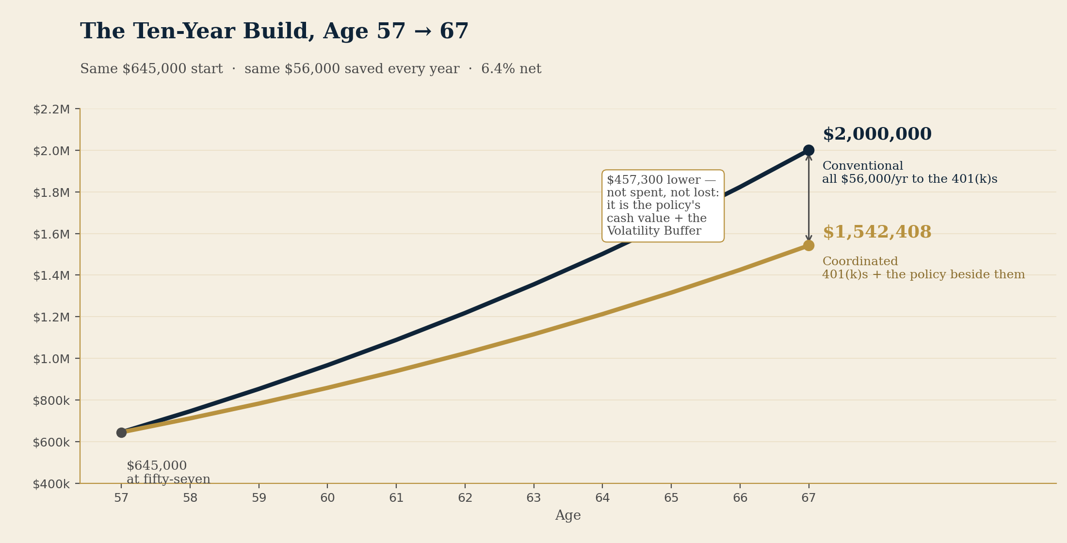
The Income-and-Legacy Scorecard
Step back from the individual exhibits, because the conventional way of comparing retirement plans measures the wrong thing and this paper needs to say what the right measure is.
A market-only plan is graded, almost always, on one number: the projected balance at some planning age. That number is a snapshot taken in the middle of a story whose ending nobody has looked at. It says nothing about whether the income survives a poor sequence, nothing about what happens if the household outlives the projection, and nothing about what is actually left when the second spouse is gone. And it invites the one comparison this whole body of work refuses — the contest of rates, in which the tempting move is to quote the return of a market sleeve against the return of an annuity and declare a winner. That contest is a category error. A plan is not a rate; it is a system that delivers income while you live and leaves something when you go. So the measure is a scorecard: what each plan delivers across a thirty-year retirement, and what it leaves.
On that scorecard, the pattern across every exhibit in this paper is the same, and it is worth collecting once:
On income. The Conventional plan delivers income only for as long as the account survives the sequence — twenty-three years in the $1,000,000 exhibit, longer in the Barrett case, but always contingent on the order the market delivered. The coordinated plan delivers baseline income for life, both spouses, by contract, regardless of the market or the calendar. The Firewall converts "income until the account runs out" into "income that cannot be outlived."
On the sequence itself. The Conventional plan meets every down year with a forced sale. The coordinated plan meets the year after a loss with the Buffer and leaves the portfolio to recover — so the same market that emptied the $1,000,000 account becomes survivable.
On the tax machine. The Conventional plan feeds every meter in Section 7 — all ordinary income, lumpy withdrawals, non-negotiable RMDs. The coordinated plan levels its taxable income, holds a MAGI-invisible source for the years that matter, and has room for Roth conversions the market-only plan never gets.
On legacy. This is the finding that most surprises readers, because it inverts the intuition. The household that removed its income from the market did not sacrifice its legacy to do so — it increased it, from $0 to $1,169,122 on an identical $1,000,000, and to 2.2–2.5× the Conventional legacy in the Barrett case. The market did not have to earn more. The coordinated plan simply kept more of what it earned and never sold at the bottom to fund a paycheck.
The scorecard is not only qualitative. Put the cleanest case — the same $1,000,000 at sixty-seven from Section 8 — into one table, scored whole:
| The same $1,000,000 at 67, scored whole | Conventional (market-only) | Firewall at the door |
|---|---|---|
| Income delivered across the window | $1,133,599, then stops | $1,200,000, and never stops while either spouse lives |
| Years of income | 23 full, a partial 24th, then $0 | all 25 in-window, then income for life |
| Left to heirs at 91 | $0 | $1,169,122 |
| Baseline income exposed to the market | all of it | none |
| Whole-plan net internal rate of return | 1.04% | ≈ 5%, and rising every year lived past 91 |
Whole-plan figures, not sleeve rates — each is the internal rate of the entire plan: every dollar in, every dollar out, the terminal value included. Drawn from Exhibits 4·A, 8·A, and 8·B.
If a household still insists on a single number, that last row is the only honest one: a whole-plan blended net internal rate of return, not the isolated return of any sleeve. For the Conventional plan it is the 1.04% of Section 4 — a million dollars in, $1,133,599 of income out, nothing left. For the Firewall plan it is the internal rate of a million dollars in, $48,000 a year out for as long as either spouse lives, and $1,169,122 remaining: taken only to age ninety-one and no further, approximately 5% — and it rises with every year lived past ninety-one, because the income does not stop while the ruler is still running. Whole against whole, the coordinated plan wins on the single number too, and wins by more the longer the household lives. The internal return of any one sleeve is still withheld, because it measures the smallest part and hides the guarantee and the legacy entirely.
Two honest conventions hold the whole comparison together: every market draw is gross, pre-tax, from tax-deferred accounts with the terminal 25% tax applied where this paper applies it — so a $48,000 draw is not $48,000 spendable and an ending balance is not spendable until its tax is paid — and every policy and annuity figure is illustrated at the carrier's current scale, quoted nearer a floor than a ceiling. Built on the conservative version of every number, the conclusion holds anyway: across income, longevity, the tax machine, and legacy, the coordinated plan is not the safer plan that gives something up. It is the better plan on every axis a retirement is measured by.
Two refinements make the scorecard fairer still, and both cut the coordinated plan's way. The gross is held equal; the spendable is not. Every comparison in this paper holds the two plans to the same $144,000 of gross income, so neither is flattered by simply drawing more. But a dollar of gross is not a dollar spent. The Conventional household's $144,000 is almost all ordinary, MAGI-counting income — it runs the full Section 7 machine, drags its Social Security into taxation, and hands the difference to the IRS before a cent is spent. The coordinated household draws the same $144,000, but a large share of it — the policy income that carries the Buffer, and the annuitized and converted balances behind the floor — arrives tax-free and invisible to provisional income, so less of the identical gross is taxable and more of it is actually spendable, and less of the couple's Social Security is dragged into tax alongside it. Section 7's two-household table priced this exactly: on one $100,000 lifestyle, the taxable income created was $92,500 on one road and $0 on the other. Same headline number, more real money — before the larger legacy is even counted.
What the $36,000 discretionary actually stands for. The case study draws a level $36,000 of discretionary income, and a careful reader will ask whether a flat figure quietly ignores inflation. It does not — it builds it in. Read the $36,000 not as a fixed lifestyle but as the twenty-five-year average of a need that starts smaller and grows: about $25,000 of discretionary and unexpected spending in the first year — travel, help for family, the larger medical bills that arrive later — rising at 3% a year. By the twenty-fifth year that same need is just over $50,000; averaged across the whole retirement it is roughly $36,000 a year. The level $36,000 was used for comparative simplicity, but it is the inflation-adjusted average of a rising real need, not a number pretending prices hold still. Section 12 takes up where the rest of the inflation adjustment lives — in the growth sleeve and in Social Security's COLA — but the discretionary figure itself already carries the raise.
Inflationthe Risk the Level Number Hides
A guaranteed income has an obvious objection, and a paper that skipped it would deserve the skepticism: a level payment loses purchasing power every year it stays level. The Firewall pays $48,000, and it pays $48,000 whether the year is 2001 or 2025. Inflation does not care that the payment is guaranteed. So the objection has to be met head-on, not waved at — and the honest answer is not that inflation is harmless. It is that a coordinated plan is built to carry it in the right place.
Start by sizing the problem honestly. At 3% inflation — near the long-run average — a dollar loses about half its purchasing power over twenty-five years: $1.00 today buys about 48 cents of goods at ninety-two. So the Firewall's level $48,000, twenty-five years on, spends like roughly $22,900 in today's money. That erosion is real, and no framing removes it. If the level annuity were the entire plan, the objection would be fatal.
It is not the entire plan, and this is where the coordination does its work. Three facts change the picture:
Most of the baseline the Firewall protects is not, in fact, level. In the Barrett household of Section 10, the $108,000 baseline is carried by four sources — and the largest, Social Security ($50,000), carries its own annual cost-of-living adjustment by law. Only the annuity-and-policy portion (about $48,000 of the $108,000) is truly fixed. Slightly more than half the "guaranteed" floor already rises with inflation before the plan does anything clever.
The inflation hedge lives, deliberately, in the growth assets. The whole point of the tier design is that the baseline is made boring and certain so that the market sleeve — which carries the discretionary $36,000 and much of the legacy — is left free to grow. Equities are the one asset that has historically outrun inflation over long horizons; the coordinated plan does not ask the guaranteed sleeve to fight inflation, because it keeps a growth sleeve whose entire job is to. And the whole life death benefit and cash value grow over time on the current dividend scale, adding a second rising line behind the level one.
A COLA rider is available — and usually the wrong trade. Annuities can be bought with a cost-of-living adjustment that raises the payment 2–3% a year. The honest catch is that the insurer prices it: a COLA rider typically lowers the starting payout by roughly a quarter to a third. A household that buys a rising payment surrenders a large share of its early income — the years it is most able to enjoy it — to protect the later years. For most households the better arrangement is to take the higher level payout as the floor and let the growth sleeve carry the raise, rather than pay an insurer to convert growth-sleeve work into a lower guarantee. It is a real choice, and a live plan runs it both ways; the point here is that "the annuity doesn't index" is not the end of the conversation, it is the start of a design decision the coordinated plan is built to make.
So the level number is not the whole story, and inflation is not an argument against the Firewall — it is an argument for holding the Firewall and a growth sleeve and a growing policy at once, each doing the job it is suited to. The market-only plan, by contrast, has no floor at all: its answer to inflation is to hope the same volatile sequence that Section 4 emptied also happens to outrun rising prices while it is being drawn down. The coordinated plan does not hope. It assigns inflation to the asset built to beat it, and certainty to the asset built to provide it.
The Two Fearsthe Dual-Risk Mechanism and Why "Guaranteed" Is Earned
There are only two ways for the money to fail a life, and every retiree knows both without being taught.
The first is that you live longer than it lasts — the account that looked like enough at sixty-seven becomes a number you watch fall, and the arithmetic of a long life turns against you exactly when you can do least about it. The second is that you go too soon — before the years you were counting on — and the people you were building it for are left with less than you meant them to have. One fear keeps a person awake; the other sits quietly underneath everything. And almost every retirement product asks you to insure against one of them by betting against the other. Buy the lifetime income and you have bet on living long; go early and you got little for it. Buy the death benefit and you have bet on going early; live long and it did nothing for the years you actually spent. Nobody wants to make either bet about their own death — which is the source of the two great objections in this whole field, "what if I annuitize and die the next year?" and "what if I skip it, live to ninety-eight, and run out?"
Here is the precise thing, and it is the deepest reason "guaranteed" is an earned word. The two instruments a coordinated plan already holds — the lifetime income of the Firewall and the death benefit behind the whole life policy — are not two products hedging two worries. They are the two halves of a single hedge, and they hedge the same variable: how long you live. The annuity's internal return is lowest if you die early and climbs the longer you live. The policy's internal return is highest if you die early and falls the longer you live. The two move in exact opposition to the same thing — your own lifespan — so a household that holds both watches its blended outcome stay nearly flat no matter when death comes. Die early: the annuity's return collapses, but the policy's is at its peak and the death benefit lands. Live long: the policy's return erodes, but the annuity soars, paying income that cannot be outlived. Held together, the two cancel, and the household's own timing — the one thing it cannot know and cannot control — stops deciding its financial outcome.
That cancellation is what earns the word. "Guaranteed" is not used in this paper as a hopeful adjective; it is used because the risk has been removed rather than bet. The most consistent mutual insurers survive for a century and three-quarters, paying without a missed year through depressions and wars, precisely because they hold these two opposing risks near fifty-fifty at scale — the death-benefit side and the lifetime-income side offsetting each other, so that what remains is the most stable series in finance. A household that holds both instruments runs a small mirror of that same machine on its own balance sheet. The full arithmetic of the cancellation — the two returns moving in opposition across every age of death, and the flat line they produce together — is modeled and isolated in the Appendix, where it can be examined without changing what this paper is. The point that belongs here in the body is not a number. It is that a coordinated plan does not ask a household to bet on its own longevity in either direction, and that the two fears every retiree carries are answered by the same structure at once. That is the deepest form of the claim: not that the coordinated plan earns more, but that it removes the one risk no rate of return could ever have covered — the risk of your own timing.
Anticipated Critiquesthe Full Gauntlet
A guaranteed-income plan draws a specific and well-rehearsed set of objections, and every one deserves its strongest form and a direct answer. What follows steelmans each.
"You lose the money to the insurer." This is the oldest objection to annuities, and for the wrong annuity it has force. The answer is structural: in a coordinated plan the Firewall is never held alone. It is paired with the death benefit, and Section 13 is the reason that pairing exists — the two instruments cancel, so the household does not forfeit its estate to secure its income. And the alternative the objection quietly prefers, keeping everything in the market, is exactly the plan that left $0 at ninety in Section 4. "You might not get it all back" is a strange complaint to raise against the one plan that leaves $1,169,122, in favor of the one that leaves nothing.
"What if I die early?" Then the joint contract has still paid both spouses for every year either lived, and the death benefit — the other half of the hedge — lands at its highest value precisely in the early-death case. The coordinated household's outcome barely moves whether death comes at seventy-six or a hundred and six; that flatness is the whole point of the Appendix. Early death is the case the death benefit is built for, which is why the two are never sold apart.
"Mortality credits are just my own money handed back to me." No — and this is worth being exact about, because it is the objection that sounds most sophisticated. If the annuity merely returned your own principal and interest, its payout could not exceed a safe self-funded withdrawal rate. It does: the joint contract in this paper pays 7.40% for life, and no self-funded account can sustain that across an unknown lifespan without risking exactly the depletion Sections 4 through 6 document. The excess comes from the pool — from the actuarial certainty that some members die early and fund the payments of those who live long. That transfer is not your own money back. It is money from a risk you cannot hedge alone and an insurer can, which is the entire reason the instrument exists.
"Annuities are illiquid — you hand over the money and lose access." For a long stretch, you do not, and Exhibit 8·A shows it: the contract carries real accessible value behind the income for well over a decade — roughly $624,000 in year one, about $354,000 by year ten — before the lifetime guarantee takes over. More to the point, only the baseline is placed behind the Firewall; the discretionary income keeps its liquidity in the market sleeve and the Buffer. Liquidity is a property of a whole plan, not of one instrument, and the coordinated plan holds more usable liquidity at ninety — when it matters — than the market-only plan, which by then holds none.
"Rates could change, so this is a bad time to lock in." The rate on a lifetime income contract is fixed at purchase for life; a household that buys today owns today's terms regardless of where rates go next. The objection is really an argument for timing the annuity market, which is the same error as timing the stock market, applied to the one purchase whose entire value is that it does not depend on timing. And the deferral option (the pre-funded build in §10.5) exists precisely for the household that wants to build the income base over years rather than commit a lump at a single moment.
"I can self-insure the whole thing with a bond ladder." This is the sharpest objection, and it fails on the one thing a ladder cannot do: pool mortality. A bond ladder built to fund income for life must be sized for the longest plausible lifespan — fund to a hundred, and hope you do not reach a hundred and three — which requires far more capital than the annuity to produce the same income, and still fails if you outlive it. The annuity's 7.40% payout against a ladder's safe yield is the mortality credit made visible: the ladder has none, because a portfolio of your own bonds cannot transfer money from the short-lived to the long-lived. A ladder is a fine tool for a defined horizon. Lifetime income is not a defined horizon, and that is exactly why only an insurer can promise it.
"A 4.8% withdrawal was too aggressive; a careful retiree is fine." Section 6 is the answer in full: lowering the draw does not make a household safe, it makes it slower to fail and quieter about the risk it still carries. The $2,000,000 household drawing a conservative 4.2% did not run out — and spent its retirement watching a falling account fund a rising share of its income. The exposure is structural at every withdrawal rate; a more careful draw does not remove it.
"You cherry-picked 2001." The opposite — 2001–2025 averaged 10.32% and was a good quarter-century, which is what makes it the honest example rather than a rigged one. Section 5 puts it inside the record of worse retiree start-years (2000, 2007, 1929, 1973, 1966), and the failure mode appears wherever a severe loss lands early. The window was not chosen to be cruel; it was chosen because it was ordinary, and it still produced 1.04%.
"Buy term and invest the difference; whole life is a poor investment." This paper does not argue whole life as an investment or on rate. The cash value's role here is the Buffer — a non-correlated reserve that lets the portfolio recover untouched — and as a replacement for the safe sleeve of a plan (the bonds, not the equities), the companion Living Asset Strategy paper documents that a properly structured policy finishes ahead of a higher-yielding bond fund on tax and structure alone: $338,635 against $230,879 on an identical $100,000 over twenty-five years, though the bond carried the higher rate (5.4% vs 5.00%). The buy-term critique is aimed at a claim this paper never makes.
"I hold Roth dollars, so your tax convention overstates the market's loss." Narrowly true and it changes less than it appears, for a reason specific to this paper: a Roth changes nothing about sequence risk. Tax treatment does not decide the order of returns. The Roth account in Section 4 would have run dry on the same schedule, because the withdrawals were still forced into falling markets. What a Roth does change is the tax machine of Section 7 — Roth income is genuinely MAGI-invisible — which is why the coordinated plan uses Roth conversions as one of its levers. The Roth helps the tax half of the problem and does nothing for the sequence half, which is the half this paper is mostly about.
"You're just afraid of the market." No — every exhibit here keeps a market sleeve, because market growth is a real and necessary engine that carries the discretionary income and much of the legacy. What the coordinated plan refuses to do is ask the market to guarantee a paycheck, which it was never built to do. The market keeps its job. It simply stops being asked to do the one job only an insurer can.
"A level guarantee gets eaten by inflation." Real, and answered in full in Section 12. The short version: a level payment does lose purchasing power, which is exactly why the coordinated plan does not assign inflation to the guaranteed sleeve. The largest piece of the baseline — Social Security — already indexes by law; the market sleeve and the growing policy carry the raise; the Firewall carries the floor. A cost-of-living rider on the annuity exists, and usually surrenders more in early income than it returns. The objection is an argument for holding the whole structure, not against the annuity within it.
"What if the insurance company fails?" The guarantee is only as good as the insurer, and that deserves a real answer rather than a wave. Two of them. First, selection: these contracts are placed with the most highly rated, long-established mutual carriers — the ones that have paid without a missed year through the Depression, two World Wars, and 2008, precisely because the offsetting dual-risk structure of Section 13 is the same machine that keeps them solvent. Second, structure: state guaranty associations backstop annuity and life obligations up to per-contract limits, and a plan sizes and splits placements with those limits in view. The risk is not zero — nothing is — but it is a smaller and different order of risk than the sequence risk it retires, and it is managed, not ignored.
"What if I need a large sum for long-term care or a health shock?" Here the coordinated plan holds more usable liquidity than the market-only plan, not less. The market-only household facing a large care bill in a down year sells depressed shares to pay it — the sequence-risk trap in its most painful form. The coordinated household draws the lump from the policy's cash value (reachable on demand, no tax event) and from the Buffer, leaving the market untouched, while the death benefit behind the plan replaces what care consumes; many properly structured policies also carry or can add a chronic-illness rider that accelerates the death benefit for care. Liquidity for a shock is a property of the whole plan, and the coordinated plan has the most of it at exactly the ages a shock is likeliest.
"I'll just work a few more years." A real lever, and nothing here argues against it — working longer shortens the drawdown, adds savings, and delays Social Security into a larger, still-indexed benefit. But it does not remove the risk this paper is about. A household that retires at seventy rather than sixty-seven still begins drawing into whatever sequence the market delivers next; it has moved the starting line, not changed the game. And the lever has a limit no one controls: health, layoffs, and the care of a spouse end careers on their own schedule, not the plan's. Working longer improves the odds. The Firewall removes the risk. They are not the same move — and the second does not depend on the first still being available when the time comes.
What This Paper Is Not Arguing
To prevent misreading, the boundaries stated plainly.
It is not arguing that anyone should leave the market. Every exhibit keeps a market sleeve; market growth carries the discretionary income and much of the legacy. The argument is about which dollar does which job.
It is not arguing that the coordinated plan wins a rate contest against the market's advertised return, and it posts no piece rate anywhere to imply otherwise. The market's advertised average is not a number anyone keeps, and refusing that comparison is not losing it. The claim is higher and safer on the whole-plan basis a retirement is actually lived on — never lesser-but-safer.
It is not arguing that every household should hold every instrument here. One that is unwilling to consider whole life, or cannot qualify, still has a coordinated plan available — the income floor built with the Firewall, the buffer approximated with cash reserves or a certificate ladder, the legacy handled through existing assets. More moving parts, sometimes less efficient, and categorically better than the unprotected plan it replaces.
It is not arguing from catastrophe. The argument is built on ordinary down years, not a crash. Where the real 2001–2025 sequence includes a severe year it is there because it actually happened — but no exhibit and no sentence reaches for a catastrophe to carry the case, because the ordinary year carries it and a catastrophe would only let the reader escape it.
It is arguing one thing: that once income begins, the order of returns is the dominant risk, that the distribution phase brings a tax machine a market-only plan is not built for, and that the two systems documented here — the Firewall, which needs no runway, and the Buffer, which must be built before it is needed — change the outcome across income, longevity, the tax machine, and legacy at once, for the households where they fit.
The Planning ConversationHow This Is Presented, and Why It Does Not Frighten
Everything in this paper could be delivered as fear, and it would be both a mistake and a misreading. A retiree told that the market kept them 1.04%, that a level guarantee erodes, and that a tax machine is waiting to tax their Social Security and surcharge their Medicare would be right to feel alarmed — and would have learned nothing they can act on. The facts are not the message. The message is the one the tier ladder already carries: this is solvable, it is solvable with money the household already has, and no one is too late. How the analysis is presented is therefore part of the analysis, and it follows a specific order.
It begins where this paper begins — not with a product and not with a crash, but with the honest benchmark: what the market actually keeps a saver, and then a retiree. A household that sees the 10.32% become 4.93% become 1.04% understands the problem before any solution is named, and understands it as arithmetic rather than salesmanship. The order matters: a conversation that leads with an instrument invites the question "what are you selling?"; a conversation that leads with the household's own numbers invites the question "what do I do about it?"
It stays with the ordinary year, never the catastrophe. The scene is always the 15% decline that demands a 24.7% recovery, because that is what actually happens and because a crash lets a person escape into "that won't be me." A planning conversation built on fear of a collapse ages badly and is easy to dismiss; one built on the arithmetic of a normal down year cannot be argued away, because the client has lived through several of them.
It presents the two protections as a ladder, not a verdict. The reader at the door is not told they missed the top rung; they are shown the Firewall they can switch on today, and told plainly what a decade of runway would have added. Nobody is scolded for the road they are already on — the Conventional plan is what almost everyone does, and it is presented blame-free. The point of the conversation is never that the household did something wrong. It is that a structure nobody designed is quietly costing them, and that structure is the one thing still in reach.
And it produces something concrete, which is the whole reason to have it. A Retirement Income Diagnostic looks at the four things this paper has treated — income, taxes, protection, and legacy — and asks one question of them together: do they work as a single system, or do they simply sit side by side. That question is almost never asked, because the people equipped to answer its parts are different people. The investment advisor manages the portfolio; the CPA files this year's return; the attorney drew up a trust years ago. Each is good at a piece. None is designing for the total, and the seams between them are exactly where the leaks in Section 11's scorecard live. The diagnostic's job is to find those seams and to design across them — principles first, then strategy, then whatever instruments the plan actually calls for, with one person responsible for the whole.
That is the conversation this paper is built to support. It is not an alarm. It is an invitation to look at the total, once, with someone whose job is the total — and to leave knowing where the seams are, whether or not anything is done about them that day.
ConclusionA Retirement That Holds Up Whether or Not the Market Cooperates
Every argument in this paper has been made in dollars, because dollars trace and survive a skeptic. But the dollars are not, in the end, what the paper is about — and the most important comparison is the one the account balances cannot show.
Imagine two households that arrive at nearly the same financial ending. Same after-tax income across retirement. Both live to the same age. They leave their children roughly the same net legacy. On a spreadsheet, a tie. And yet they did not live the same retirement — and the difference is not a feeling a rigorous paper has to wave at. It is measurable, and it reduces to three quantities the exhibits above already established. The first is the variance of their income: one household's baseline income moved with the market every year; the other's did not move at all, because it had been removed from the market's jurisdiction by contract. The second is the probability of depletion: for one household that probability was real — Section 4 is what it looks like when it lands — and for the other it was zero on the baseline, by the terms of the Firewall. The third is the dispersion of the legacy across the timing of death: one household's legacy swung on the order of returns and the length of its life; the other's, holding the two halves of the single hedge in Section 13, stayed nearly flat regardless of when death came. Three measured quantities — zero-or-flat for the coordinated household, open-ended for the Conventional one — and all three describe the same thing from different angles: the two fears every retiree carries, running out too soon and leaving too little behind, present in one retirement and absent from the other.
That is where this paper stops, deliberately. It would be easy, and a mistake, to add the sentence about how the coordinated family therefore slept better, traveled without checking the market first, helped a grandchild without recalculating whether they could afford to. Those things are almost certainly true, and they are exactly the sort of claim a rigorous analysis must not make, because they cannot be measured and the moment they are asserted the whole edifice is dismissed with a line — you can't put a number on that. So the paper does not assert them. It proves the risk was removed, names the two fears the removal answers, and lets the reader supply the rest. The math is the relief. It does not need to be narrated to be felt.
And the plan does one more thing, which is the reason it completes rather than merely lasts. The death benefit behind the coordinated plan is not an afterthought to the income — it is what lets a retiree spend confidently in the first place, because whatever is not spent is replaced, and it is what resets the next generation's starting line rather than handing them a remainder. Every ordinary way of building wealth depends on a clock no one controls: you must live long enough to finish, and long enough for it to grow. The single event that breaks every other plan — an early death — is the event this structure is built to complete on schedule, from the day it is in force. That is where this paper hands off to the rest of the system. The Accumulation series proved what disciplined growth is actually worth once the market's four forces have taken their share; the Living Asset Strategy proved what a single dollar can do when it is never interrupted; and the Distribution series has proved what both become when the paychecks stop and the money has to last. Read together, the three describe one coordinated life — accumulated honestly, deployed without interruption, and distributed so that it holds up whether or not the market cooperates, and completes whether the years are many or few.
The transformation this points toward is not, finally, a product or a rate. It is the difference between a retirement that depends on the market behaving and one that does not — between a bad market in the second year of retirement being a personal crisis or merely a news story. That is what a coordinated Retirement Income Plan is for, and it is worth building before the fact, while the pieces can still be positioned, because the worst time to discover a plan has one protection instead of two is the year both are needed.
Where to begin. The clearest first step is a Retirement Income Diagnostic — a focused look at how your money is actually put together: whether your income, your taxes, your protection, and your legacy work as one system or just sit side by side. You leave knowing where the seams are, whether or not you do anything about them. What it produces is a coordinated Retirement Income Plan — principles first, then strategy, then whatever instruments the plan actually calls for, with one person designing for the total. Every figure in this paper belongs to an illustration. The ones that matter belong to you.
Nate Butler · Retirement Income Specialist · Forte Life
nbutler@fortelife.net · 801-997-6861 · calendly.com/nbutler-fortelife
Certainty · Liquidity · Legacy
Methodology and Disclosures
Market figures. All market figures are measurements of the actual S&P 500 total return, not projections, run through the Forte Life Cash Flow Calculator and presented as that engine's exported output. The primary worked window is 2001–2025 (arithmetic mean 10.32%; twenty of twenty-five years positive). Order-independence in accumulation is confirmed both algebraically (the product of annual factors is commutative) and empirically (random permutations of a historical sequence produce identical ending balances). All market scenarios assume the tax-deferred convention established in the companion Accumulation paper and summarized in Section 2 here: a 25% terminal rate (20% federal + 5% state), a 1.00% all-in fee, 1.50% Activity Drag, negative balances not permitted.
The sequence-risk record (Exhibits 5·A and 5·B), traced. Six retiree start-years, $1,000,000 · −$48,000/yr · four forces, each run market-only and with the Firewall, every account floored at zero (no negative balances). The annuity contract terms (7.40% joint lifetime payout) are held constant across all start-years by design — anachronistic for the earliest years and intentionally so — varying only the market sequence; a start-year without a full 25-year window runs forward to 2025 and then repeats from its own start to fill the remainder (2007 → 2025, then 2007–2012). Market-only — income paid before depletion, then ending: 1929 $540,146 (income stops age 78) → $0; 2000 $833,781 (stops 84) → $0; 2001 $1,133,599 (stops 90) → $0; 2007 $1,200,000 (survives) → $749,483; 1966 $1,200,000 (survives) → $658,787; 1973 $1,200,000 (survives) → $2,254,159. Firewall — $1,200,000 income across the window (continuing for life), then remainder ending: 2000 $899,565; 2001 $1,169,122; 2007 $1,127,838; 1929 $505,071; 1966 $1,396,991; 1973 $3,099,539. Exhibit 5·B holds the 2001 household four ways, changing only fixed-vs-variable: fixed 10.32% market-only $1,200,000/$2,099,631 and Firewall $1,200,000/$1,695,589; variable market-only $1,133,599/$0 and Firewall $1,200,000/$1,169,122. Firewall figures are income delivered and remainder ending (scorecard), never posted as internal rates.
No piece rates. The internal rate of return of any single sleeve of a multi-part plan (a market remainder, an annuity alone) is never posted. Whole-plan comparison is by the income-and-legacy scorecard, or by a whole-plan blended net IRR computed on the calculator; the only rates printed are whole-plan figures — the Conventional plans' 1.04% and 2.28%, and the Firewall plan's whole-plan blended net IRR of approximately 5% shown in Section 11 (a rate on the entire plan, every dollar in and out, not on any sleeve) — together with the isolated dual-risk structure of the Appendix, which carries its own isolation statement.
Buffer sizing. Across the 76 rolling 25-year windows of 1926–2025, the longest unbroken run of down years had a median of two and a maximum of four (1929–1932); a three-year buffer covers 72 of 76 windows, four covers all 76. Stated range: three to five years, sized to cover the longest unbroken run and nothing beyond it.
The ordinary-year illustration. $1,000,000, $48,000 drawn, a 15% decline: $1,000,000 → $850,000, less $48,000 → $802,000, requiring a 24.7% gain to return to $1,000,000.
Inflation. The purchasing-power illustration in Section 12 uses a 3% long-run inflation assumption — under which a dollar retains roughly 48 cents of purchasing power across twenty-five years — to size the erosion of a level payment; the coordinated response (Social Security's statutory cost-of-living adjustment on the largest baseline component, the growth sleeve and the growing policy carrying the real adjustment, and the priced cost of an annuity cost-of-living rider) is directional, not a projection.
Four Forces and bond-replacement hand-backs. The four-force derivation and the 6.40% median / 4.93% window are the companion Accumulation paper; the bond-replacement figures ($338,635 vs $230,879 on $100,000 over 25 years) are the companion Living Asset Strategy paper. Cited as results; not re-derived.
Tax-machine figures. Provisional-income thresholds ($32,000 / $44,000 married-filing-jointly), the 50%/85% inclusion, the torpedo multipliers (1.5×/1.85×), the IRMAA cliff structure and two-year lookback, and the RMD age are current published statutory and regulatory rules, not calculator outputs; exact IRMAA thresholds and surcharge amounts are published annually and a live plan uses the current figures. The provisional-income thresholds are not indexed to inflation; this is stated because it is a load-bearing point. The worked household examples in Section 7 — the $10,000-draw torpedo, the $206,000 IRMAA cliff, the Uniform Lifetime RMD schedule on a $1,000,000 balance, and the two-household $100,000-lifestyle MAGI comparison — apply these current statutory rules to illustrative households; the date-sensitive dollar amounts (the 2025 IRMAA tiers of $74.00 Part B and $13.70 Part D per person, and the RMD divisors) are current-year figures updated annually, while the mechanisms they show are permanent.
Guaranteed-language reservation. "Guaranteed" is used only for contractual lifetime income and a policy's contractual floor, never for dividends, illustrated values, or market performance. Policy and annuity values reflect current illustrated scales and are not guarantees of future results; guarantees rest on the claims-paying ability of the issuing carrier. Carriers are named generically in this educational context.
This whitepaper is produced for educational and informational purposes only. It does not constitute investment, tax, insurance, or legal advice. Individual circumstances vary. Past performance is not indicative of future results. Guarantees are subject to the claims-paying ability of the issuer. Consult qualified professionals before making financial decisions.
© 2026 Forte Life. All rights reserved.
The Dual-Risk Capstone, Isolated
This appendix isolates the guaranteed layer of a coordinated plan and measures a single thing: what holding both a lifetime income and a death benefit does to the risk of your own timing. The market growth sleeve is absent here — not because it is unwanted, but because it is not what is being measured, exactly as the companion Living Asset Strategy isolates a bond sleeve to measure a bond replacement. Read this as a measurement of one layer, never as a recommendation to hold only that layer.
The structure modeled is insurance-only: a $500,000 lifetime income annuity paired with a whole life policy funded at $17,120 a year — the two halves of the hedge in Section 13, and nothing else. Its blended internal rate of return is computed across every age of death, so the question "what does my outcome depend on?" can be answered directly. On the carrier's current dividend scale:
| Age at death | Annuity alone | Policy alone | Blended (both held) |
|---|---|---|---|
| 80 | 4.03% | 12.47% | 6.78% |
| 85 | 4.05% | 7.19% | 5.33% |
| 86 | 4.14% | 6.62% | 5.18% (trough) |
| 90 | 5.56% | 5.11% | 5.37% |
| 95 | 6.55% | 4.20% | 5.52% |
| 100 | 7.10% | 3.71% | 5.57% |
| 107 | 7.52% | 3.71% | 5.71% |
From the modeled dual-risk exhibit, current dividend scale.
Read the two outer columns and then the middle one. Across twenty-three years of lifespan variance the annuity's return climbs 3.5 points and the policy's falls 8.8 points — enormous, opposite swings — while the blended result moves just 53 basis points (5.18% to 5.71%). The household barely feels a lifespan difference that would swing either instrument held alone. And the weak point is a shallow dip at age eighty-six — the year the annuity's own death benefit reaches zero — after which the blended figure rises, so the structure's worst case is a gentle trough, not a cliff.
The stronger version of the result survives the hardest question anyone can ask — what if the dividends are cut? — because it does not depend on dividends at all. On the contractual guaranteed scale, the blended IRR is a flat 4.14% from age eighty clear through age one hundred (28 basis points across twenty-seven years), improving only after the policy is paid up. A hard floor, dead flat across the entire plausible range of lifespans. Both fears answered by the same table: die at eighty-six and the estate collects while the plan still returns 5.18%; live to one hundred and the household has drawn a lifetime of income and still leaves a legacy at 5.57%. Neither is a bad outcome — which is precisely the claim. (Two conditions travel with the exhibit: the current-scale figures use the non-guaranteed dividend scale, and both runs assume both spouses die the same year, which a survivorship design makes reasonable but which is a simplification. The guaranteed-scale run answers the dividend objection before it is raised. The full age-by-age treatment, built to be felt rather than audited, is reserved for a standalone piece.)